Techniques Used for Measuring Work | Industries

This article throws light upon the top seven techniques used for measuring work. The techniques are: 1. Analytical Estimating 2. Predetermined Motion Time System (P.M.T.S) 3. Method-Time-Measurement (M-T-M) 4. Work Factor 5. Activity Sampling, Ratio-Delay Study or Work Sampling 6. Use of Time Study Data in Wage Incentive and Collective Bargaining 7. Ergonomics.

Technique # 1. Analytical Estimating:

Setting the time standards for long and non-repetitive operations by Stop Watch Method are uneconomical.

Analytical Estimating technique determines the time values for such jobs either by using the synthetic data or on the basis of the past experience of the estimator when no synthetic or standard data is available. In order to produce accurate results the estimator must have sufficient experience of estimating, motion study, time study and the use of synthetised time standards.

BS 3138:

1969 defined Analytical Estimating as a Work Measurement technique being a development of estimating, whereby the time required to carry out elements of a job at a defined level of performance is estimated partly from knowledge and practical experience of the elements concerned and partly from synthetic data.

Procedure of Analytical Estimating:

The various procedural steps involved in Analytical Estimating are:

(a) Find out job details which include job dimensions, standard procedure and especially the job conditions, i.e., poor illumination, high temperatures, hazardous environments, availability of special jigs, fixtures or tooling’s, condition of materials or other parts to be operated upon, etc.

(b) Break the job into Constituent elements.

(c) Select time values for as many elements possible from the library of element time values (i.e., synthetic data).

(d) To the remaining elements for which no synthetic data is available, usually the estimator gives suitable time values from his past knowledge and experience.

(e) Add (c) and (d) and this is the total basic time at a 100% rating.

(f) Add to (e) an appropriate Blanket Relaxation Allowance. In analytical estimating, Relaxation Allowance is not added to individual elements, rather a blanket, R. A., depending upon the type of job and job conditions, is pre-decided as a percentage (10-20%) of the total basic time and is added to the total basic time.

(g) Any additional allowances if applicable may be added to (f) in order to arrive at Standard Time for the given job or task.

Advantages  of Analytical Estimating:

(i) It possesses almost the same advantages as enjoyed by synthesis technique of Work Measure­ment.

(ii) It aids in planning and scheduling.

(iii) It provides a basis for rate fixing for non-repetitive works in industries.

(iv) It improves labour control.

Drawback of Analytical Estimating:

Since analytical estimating relies upon the judgment of the estimator, the time values obtained are not as accurate and reliable as estimated by other work measurement techniques.

Uses or Applications of Analytical Estimating:

Analytical estimating is used,

(i) For non-repetitive jobs, jobs involving long cycle times and the jobs having elements of variable nature. Stop watch time study or building synthetic data, for timing such jobs does not prove to be economical.

(ii) In Repair and Maintenance work,

Tool rooms,

Engineering construction,

Job production,

One time large projects, and

Office routines, etc.

Difference between Synthesis, P.M.T.S. and Analytical Estimating:

Synthesis, P.M.T.S, or Analytical Estimating, all these techniques estimate the standard time of a job without themselves measuring the time, i.e., these techniques do not employ a time measuring equipment like stop watch, etc.

(i) Synthesis builds up the total time for a job by adding the times for different elements of the job. The element time values are taken from a catalogue (of elements times) built from a firm’s own past time studies on other jobs having the concerned elements. Time values for all the elements of a job to be timed can be found from the previously collected lime data, (Synthetic Data).

(ii) P.M.T.S. is similar to synthesis but differs as regards the characteristics of the job elements. P.M.T.S. deals with more basic elements of duration 0.1 second or less whereas the element time in case of synthesis may be of 3 to 4 seconds of duration.

Like Synthesis, P.M.T.S. also relies upon manuals or time catalogues for building the total time for a job.

(iii) Analytical Estimating differs from P.M.T.S. as regards the duration of elements. It is similar to synthesis.

Analytical Estimating differs from synthesis in the sense that it estimates time of non-repetitive and long operation jobs, for whose all job elements, past time data may not be available with the firm. Hence the time for the new job has to be determined, by timing some elements on the basis of synthetic data available and the remaining elements are given a time by the estimator from his past experience of timing different jobs.

Technique # 2. Predetermined Motion Time System (P.M.T.S):

An element in Macro data, e.g., pick up the screw driver may have its timed value of several seconds whereas in Micro data the elements of the job are basic human motions with duration 0.1 second or even less. This section will deal with M-T-M and Work Factor Systems (i.e., PMTS) which are known as Micro data. Micro data is based upon much smaller division of motions (i.e., therbligs) as compared to Macro data.

BS 3138:

1969defines PMTS as a work measurement technique whereby times established for basic human motions (classified according to the nature of the motion and the conditions under which it is made) are used to build up the time for a job at a defined level of performance.

Technique of PMTS:

i. The technique to build PMTS data does not measure element time by a stop watch and thus it avoids the inaccuracies being introduced owing to the element of human judgement.

ii. It is assumed that all manual tasks in industries are made up of certain basic human movements (like reach, move, disengage etc.) which are common to almost all jobs.

iii. The average time taken by the (normal) industrial workers to perform a basic movement is practically constant.

With the above facts in mind, the various steps involved in collecting PMTS data are as follows:

(a) Select large number of workers doing varieties of jobs under normal working conditions in industries.

(b) Record the job operations on a movie film. (Micromotion study).

(c) Analyse the film, note down the time taken to complete each element and compile the data in the form of a table or chart.

The jobs selected are such that they involve most of the common basic motions and are worked under different set of conditions by workers having different ages and other characteristics.

Once the tables for various basic motions are ready, the normal time for any new job can be determined by breaking the job into its basic movements, noting time for each motion from the tables and adding up the time values for all the basic motions involved in the job.

Standard time may be obtained by adding proper allowances.

Objects and Uses of PMTS:

Predetermined motion time system finds the following uses:

(i) It is very useful in Method Analysis.

(ii) It helps modifying and improving work methods before starting the work on the job.

(iii) It sets time standards for different jobs.

(iv) It assists in constructing time formulae.

(v) It aids in the pre-balancing of the manufacturing lines.

(vi) It provides a basis for wage plans and labour cost estimation.

(vii) It facilitates training of the workers and supervisor.

(viii) It is used for timing those short and repetitive motions which cannot be measured by stop watch.

Advantages of PMTS:

Predetermined motion time system possesses the following advantages:

(i) It eliminates inaccuracies associated with stop watch time study.

(ii) It is superior to stop watch time study when applied to short cycle highly repetitive operations.

(iii) Time standard for a job can be arrived at without going to the place of work.

(iv) Unlike stop watch study, no rating factor is employed.

(v) PMTS data, since it is the result of very large number of observations, is more reliable and accurate as compared to stop watch time study data.

(vi) The time and cost associated with finding the standard time for a job is considerably reduced.

(vii) Alternative methods are compared easily.

(viii) PMTS helps in tool and product design.

Drawbacks of PMTS:

(i) PMTS can deal only with manual motions of an operation.

(ii) All categories of motions have not been considered while collecting PMTS data.

Applications of PMTS:

Predetermined motion time system is usefully employed for the following types of jobs:

(a) Machining work,

(b) Maintenance work,

(c) Assembly jobs,

(d) Servicing, and

(e) Office work.

Technique # 3. Method-Time-Measurement (M-T-M):

This system was developed by Method-Time-Measurement Association and it got recognition in 1948. Unlike work factor system, M-T-M does not require any modification of the basic time values. Moreover the basic human movements in this system are analysed in more detail. M-T-M measures time in terms of TMUs (Time-Measurement-Units) and 1 TMU = 0.0006 minutes.

M-T-M analyses an industrial job into the basic human movements required to do the same. From the tables of these basic motions (Table I to IX), depending upon the kind of motion, and conditions under which it is made, predetermined time values are given to each motion. When all such times are added up, it provides the normal time for the job. Standard time can be found by adding suitable allowances.

According to M-T-M the various classifications of motions are:

(i) Reach-R,

(ii) Move-M,

(iii) Turn and Apply Pressure-T and AP,

(iv) Grasp-G,

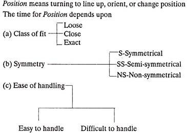
(v) Position-P,

(vi) Release-RL,

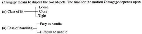
(vii) Disengage-D,

(viii) Eye travel time and eye focus time-ET and EF.

(ix) Body, Leg and Foot Motions, and

(x) Simultaneous Motions.

A table is provided for each motion. Depending upon different characteristics of a motion, the time can be read from the table.

In Reach the hand moves to destination and has a predefined objective.

Time for Reach depends upon:

(i) The distance moved,

(ii) Nature of destination,

(iii) Type of reach, (i.e., whether hands move/accelerate/decelerate at the beginning/end of reach or not).

There are five cases for the motion Reach:

A. Reach to an object in other hand or to an object in fixed location.

B. Reach to single object in location which may vary a little from cycle to cycle.

C. Reach to object jumbled with other objects in a group. It involves search and select.

D. Reach to a very small object or reach to an object where accurate grasp is required.

E. Reach to indefinite location to get hand in position for body balance.

Move involves transporting an object to a definite location.

Time for Move is influenced by:

(i) Nature of location or destination,

(ii) Distance moved,

(iii) Weight factor (or resistance), and

(iv) Type of move.

There are three cases for the basic motion Move:

A. Move object to other hand or against stop.

B. Move object to approximate or indefinite location.

C. Move object to exact location.

Apply pressure case 1: 16.2 TMU

Apply pressure case 2: 10.6 TMU

Turn indicates the rotation of the hand about the axis of forearm.

The time for Turn depends upon the degrees turned and the weight factor. Weight factor classifies Turn into three types namely Small, Medium and Large (refer Table-Ill)

Apply Pressure means the application of pressure to:

(i) Squeeze an object say a lever,

(ii) Overcome resistance-It requires more force than (i).

Grasp means taking hold of an object. Motions like Search and Select precede Grasp. The time for Grasp depends upon the description or type of the grasp motion.

Technique # 4. Work Factor:

Work Factor System got developed in Philadelphia in the year 1934. The two main names associated with Work Factor System were those of J. H. Quick and W. J. Shea. Like M-T-M, Work Factor System,

(i) Also relies on manuals containing time values for different elements (i.e., leg, trunk, foot, etc.) predetermined from high speed films of a large number of Industrial Operations. Unlike M-T-M, Work Factor System,

(i) Is more accurate,

(ii) Has a simple and easy procedure,

(iii) In addition to other aspects, it takes into account Mental Process Times,

(iv) Considers some non-productive times also,

(v) Has its standards for an experienced skilled worker whereas M-T-M standards are based upon the performance of an average operator. Because of this reason, for the same job, Work Factor System gives a smaller time as compared to M-T-M.

(vi) Has 1 Time Unit = 0.0001 minutes.

Classification of Work Factor:

Work Factor System has a number of sets of data. For example:

1. Detailed Work Factor:

(a) As the name suggests, it is detailed for fine analysis.

(b) It is preferred for high accuracy and consistency of results.

(c) It is used for cost reduction, method improvement and setting time standards.

(d) It cannot be applied (used) by an untrained personnel.

2. Simplified Work Factor:

(a) It involves broader elements and provides quicker results.

(b) It is not so precise as the Detailed Work Factor.

(c) The error in the results obtained by this system may be of the order of 0.5%.

(d) It may be used for timing-machining, maintenance and material handling operations.

(e) Like Detailed Work Factor, it is also employed for estimating cost of different operations.

3. Abbreviated Work Factor:

(a) It is the further abbreviation of the Work Factors explained above.

(b) It provides still quicker analysis.

(c) It is not so precise as the Detailed or Simplified Work Factor.

(d) The standard time estimated by this system is more than that found out by Detailed or Simplified Work Factor.

(e) Unlike the two Work Factors explained above, the Abbreviated Work Factor possesses all the data in one sheet.

(f) It finds applications in construction work, maintenance and material handling operations.

4. Ready Work Factor:

(a) As compared to all other Work Factor Systems, it is easy to learn and to administer.

(b) It is meant for persons (belonging to other departments like accounts, etc.) which do not have much experience of Work Study.

The Detailed Work Factor is discussed below:

Principle of Work Factor:

Detailed Work Factor considers some basic motions whose time in turn is modified by the elements of difficulty, (i.e., the time increases in some proportion as the number of difficulties increase). As it will be explained below, weight, change of direction, etc., each factor is called a Work Factor. The more the number of Work Factors (up to 4 only) the more is the time taken for a motion.

The Detailed Work Factor considers the following:

(i) Elements of Work:

(a) Assemble,

(b) Dissemble,

(c) Grasp,

(d) Mental Process,

(e) Preposition,

(f) Release,

(g) Transport, and

(h) Use.

(a) Assemble. Putting objects together.

(b) Dissemble. Separating different parts of a body.

(c) Grasp. Taking hold of something.

(d) Mental Process. In mental process, the senses receive a stimulus and react accordingly. Sort, inspect, recollect etc., involve mental process.

(e) Preposition. Locating an article in predetermined position so that it’s ready for use.

(f) Release. Releasing or letting go an object.

(g) Transport. Moving an article or hand from one place to another.

(h) Use. Manipulating or causing a tool to do its function.

(ii) Variables of Distance:

Distances moved from 1 to 40 inches and the related times are given in Work Factor Tables.

(iii) Weights or Resistance (W):

Weights associated with the motions or the resistance experienced by a limb in performing a motion are duly accounted for in Work Factor. Besides other variables, the amount of weight (in lbs.) associated with a motion (for a male or female worker) specifies the number of Work Factors (refer W.F. Tables).

A Work Factor means an element of difficulty. An operation having 4 Work Factors associated with it implies that it is more difficult than the operation with 1 Work Factor only and thus the time associated with the former is also more [refer Table 1].

W. F. Tables also show that for each body member for a particular distance moved there are five values of times-one basic time value and the remaining four values of times depending upon the number of Work Factors associated with the motion. The basic time value is for the minimum difficulty.

(iv) Degree of Control:

The degrees of control as connected with manual work are:

a. Steering or Directional Control (S).

b. Change of Direction (U).

c. Precaution or care (P).

d. Manner of Terminating the Motion (D-Definite stop).

These categories when combined with weight classifications decide the number of Work Factors (difficulties) associated with a body motion.

(v) Body Members:

They are:

(a) Aim (4),

(b) Leg (L),

(c) Trunk (7),

(d) Finger-Hand (F, H),

(e) Foot (FT),

(f) Forearm swivel (FS).

W. F. Tables (i) to (vi) provide time values for motions connected with them.

Procedure:

The various steps involved in finding the operation time are as follows:

(a) Analyse the job in detail into individual motions,

(b) Determine the number of work factors associated with each motion.

(c) Find the time for each motion from the tables provided,

(d) Add times for all the motions, and

(e) Add the appropriate allowances to arrive at the standard time

 

Advantages:

Besides those listed earlier work factor possesses one more major advantage that-since the job is analysed in detail, bad methods prevailing in the activity are uncovered automatically.

Applications:

Work factor finds applications in:

(i) Industries making small, light hand assemblies, and

(ii) Electronic industry.

Example 1:

Using the Detailed Work Factor, find the time required in picking up a shaft of 2 inch diameter, weighing 7 lbs. from a distance of 12 inches and then placing its one end inside the bush bearing (clearance fit). Assume a male worker.

Solution:

(1) Reach to grasp the shaft. For this motion the Analysis is A12WD.

(a) A 12 means Arm motion of 12 inches.

(b) W is there because a weight of 7 lbs. and up and less than 13 lbs. adds 1 Work Factor. [Table (i)].

(c) D indicates a definite stop for the arm and therefore introduces 1 Work Factor.

From Table – WF-ARM(A) (i) for 12 inches distance and 2 Work Factors the Time Units are 85 …(i)

(2) Grasp the shaft. For this motion, the analysis is F 2. For Finger motion of 2 inches and a weight of 7 lbs. from Table (iv), the time units are 38, …(ii)

(3) Move shaft by a distance of 12 inches and then place into the bearing. For this motion, the Analysis is A 12 WSD; w is because of 7 lbs, of weight, S-due to steering of shaft end to the bearing and D -because shaft (or arm) will come to definite stop over the bearing.

Referring Table (i) ARM, the time units for a distance of 12 inches and three Work Factors, are 102. …(iii)

Therefore total time units = (i) + (ii) + (iii)

= 85 + 38 + 102 = 225

Since 1 time unit = 0.0001 minutes, thus the total time for the existing work.

= 0.0001 x 225 = 0.0225 minutes

Technique # 5. Activity Sampling, Ratio-Delay Study or Work Sampling:

L.H.C. Tippett developed Activity Sampling in Britain in 1934 for the British Cotton Industry Research Board. R. L. Morrow used this technique in America round about 1945 and named it Ratio Delay Study. In 1952, C. L. Brisley renamed the technique as Work Sampling and today it is one of the very common techniques of Work Measurement.

Activity sampling as defined by B.S. 3138: 1969, is a technique in which a large number of observations are made over a period of time of one or a group of machines, processes, or workers. Each observation records what is happening at that instant and the percent of observations recorded for a particular activity or delay is a measure of the percentage of time during which that activity or delay occurs.

Work Sampling can tell what percentage of the working day, a person spends how, i.e., for how much time he works, what time he expends for his personal needs and for how long he remains idle.

Activities of very long duration (such as to find the actual working time of an operator in one shift of eight hours) cannot be economically timed with the help of stop watch time study. In such cases, the most appropriate technique of Work Measurement is Work Sampling which takes only 1/20th of the time required for stop watch study and gives the results with an accuracy of ±2%.

Theory/Principle:

Work sampling relies upon Statistical Theory of Sampling and Probability Theory. Normal Frequency Distribution and Confidence Level are associated very much with Work Sampling.

Statistical theory of sampling explains that adequate random samples of observations spread over a sufficient period of time can construct an accurate picture of the actual situation in the system. Approximately 500 observations produce fairly reliable results and the results obtained through obser­vations 3000 or more are very accurate.

Normal frequency distribution (Fig. 9.17) portrays graphically the probability of occurrence of a chance event. Moreover, it gives important relationship between the number of standard deviations and the area under the curve representing the confidence level of an occurrence.

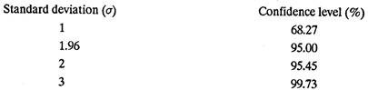
A confidence level of 95.45% signifies that the Work Study Engineer is sure that 95.45% of the times, the random observation will represent the true facts.

If the Work Study Engineer takes 25 rounds of the Machine Shop in a day, observes an operator ‘x’ and finds that

15 times he was working on the machine,

4 times he was setting up or cleaning the machine,

3 times he was not doing anything.

3 times he had gone for his personal needs; it shows that the worker spends 60% of his time in actually working over the machines and for 12% of the total time he is idle, etc., etc. These facts can be confirmed or refuted by conducting more number of observations.

Procedure:

(a) Define the problem, i.e., determine the main objectives and define each activity to be measured.

(b) Make sure that all the persons connected with the study (i.e., workers and supervisor) understand the objectives of the study.

(c) State the desired accuracy limits for the ultimate results.

(d) Conduct a Pilot Study to;

(i) Estimate the approximate percentage occurrence of the activity (i.e., p).

(ii) Estimate the required number of observations for the desired accuracy set, and

(iii) Ensure that workers have become habituated to the visits of the work study engineer.

(e) Design the actual study.

(f) Using the data obtained from Pilot Study (d)(i), above, i.e., value of p, calculate the number of observations to be made.

Example 2:

Pilot Study showed the percentage of occurrence of an activity as 50%. Determine the number of observations for 95% confidence level and an accuracy of ±2%.

Solution:

N = 4p(100-p)/L₂

where N is the number of observations

p is % of occurrence

L is limits of accuracy.

Therefore N = 4 x 50(100-50)/2² = 2500

(a) Other methods for finding number of observations are:

(1) Rule of 1000.

(2) Rule of thumb tables.

(3) Alignment charts (Fig. 9.18)

(4) Use of Random number tables.

A random number table may look like:

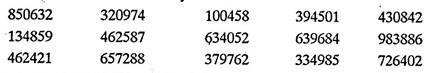
The number 850632 may imply 8.50 o’clock and 6.32 o’clock for taking an observation. A number which does not give time value in a particular shift hours may be left.

(5) Use of Punched Cards.

(b) Decide the number of days for study and select the shifts for the same.

(c) Decide the time interval between observations and the path to be followed for recording the same.

(d) Design the observation record sheet (Fig. 9.19).

(e) Make the observations and note down the information.

(f) Plot the data collected every day on the control chart. The observed data falling outside the control (3σ) limits on any day indicates an abnormal situation on that day and it may be caused out.

(g) Check the accuracy of data or the actual limit of error at the conclusion of the study.

Example 3:

2500 observations were conducted and it was found that the activity under study occurred 1200 times; determine the limits of accuracy and limits of error.

Solution:

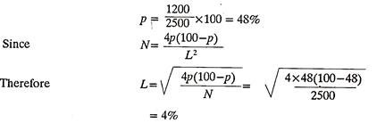
Limits of error = 48 ± 4%, i.e., in between 52% and 44%.

(—) Construct a final report, state conclusions and make recommendations, if any.

Example 4:

A work sampling study was conducted for 100 hours in the machine shop in order to estimate the standard time. The total number of observations recorded were 2500, No working activity could be noticed for 400 observations. The ratio between manual and machine elements was 2:1. Average rating factor was estimated as 1.15 and the total number of articles produced during the study period were 6000.

Rest and personal allowances may be taken as 12% of the normal time.

Solution:

Proportion of working time = 2100/2500 x 100 = 84%

Time taken to make one article = 100 x (84/100) x 60/6000 minutes

= 0.84 minutes

Out of 0.84 minutes, the time devoted by

manual labour = 0.84 x 2/3 = 0.56 minutes

and-Machine time = 0.84 x 1/3 = 0.28 minutes

Normal time per article = Observed time x Rating + Machine time.

= 0.56 x 1.15+0.28

= 0.924 minutes.

Standard time per article = Normal time + Allowances

= 0.924 + 0.924 x 12/100

= 1.0348 minutes.

Advantages:

(i) It involves much less cost as compared to stop watch time study.

(ii) It can be carried out with little naming.

(iii) It can time long operations which are almost impractical to be measured (i.e., timed) by stop watch time study.

(iv) It is very advantageous for timing group activities.

(v) It does not need any timing device like stop watch or microchronometer, etc.

(vi) Even if the study gets interrupted in between, it does not introduce any error in the results.

(vii) Observations can be made within the desired accuracy.

(viii) Large number of observations extended over days/weeks damp down the influence of day-to-day fluctuations on the results.

(ix) It can increase efficiency by uncovering the sources of delay.

Limitations:

(i) It is uneconomical both as regards time and money to study activities of short duration by Work Sampling.

(ii) It is also uneconomical in case one worker or one machine is to be studied.

(iii) It does not break, the job into elements and thus does not provide element details.

(iv) It does not assist in improving work method.

(v) It normally does not account for the speed at which an operator is working.

(vi) Workers may not understand the principles of work sampling and hence may not trust it.

(vii) Observations, neither random nor sufficient in number may produce inaccurate results.

Applications/Uses:

(i) To determine working time and idle time of men and machines.

(ii) To time long duration activities which are regular/irregular, frequent/infrequent.

(iii) To estimate the time for which material handling equipment are actually operating in a day.

(iv) To estimate allowances for unavoidable delay.

(v) In describing resource utilisation patterns.

(vi) For the purpose of cost control and accounting.

(vii) In estimating the percentage utility of the inspectors and time standards for indirect labour.

(viii) In stores, hospitals, warehousing, offices, farm work, repair and maintenance work, textile industry, machine shops, etc.

(ix) It is preferred when the cost of using other work measurement techniques tor timing a job appears to be great.

Synthesis of Work Study Data:

Work study data or in other words time study values of elements obtained from direct time studies, conducted on various jobs having different parameters and under different conditions are synthesized in order to obtain ‘Synthetic Times’ or ‘Basic Data’ or ‘Standard Data.

Before describing the procedure for synthesis of work study data, it is better to understand the meaning of synthesis. Synthesis is a work measurement technique to build up normal time for a new job (at a defined level of performance) by adding element times collected from previously held time studies on similar jobs having same elements as possessed by the new job.

The following steps are involved in synthesis:

(1) Collect all the possible details about the job, for example, material, dimensions, method, conditions, etc. The collected details should be reliable.

(2) Break the job into constituent elements. The size of the elements should be decided critically. A smaller element will have much wider range of usefulness and applicability but the time study Engineer will naturally take longer time to compile the standard time for the job.

Three types of elements, namely machine elements, constant elements, and variable elements may be there, in a job.

Machine Elements:

They are controlled by the characteristics of the process such as feed, speed, depth of the cut, amount of metal to be removed, etc.

Constant Elements:

They are identical from job to job; for example, mounting a cutter on the milling machine arbor or holding a lathe tool in the tool post.

Variable Elements:

They are similar in nature from job to job but vary in difficulty and the time required to complete them, because different jobs may possess different dimensions, shapes, and weights. Variable elements may be those, involving hand work or others, influenced by the changes in metal machinability, quality, tolerances, etc.

Constant, variable or machine elements in each job, may be repeated the same number of time, different number of times or they may or may not be present in various jobs.

Constant elements are easy to deal with. Only sufficient number of observations are required to obtain a realistic time. Variable elements are quite problem us as compared to constant elements and need more skill and attention on the part of analyst. Good number of observations are must in order to establish a relationship (which may be a straight line or a curve) between the element characteristics and basic time for that element.

Machine elements are normally calculated from the information, of speed of job rotation, feed of the tool and the depth of cut, etc.

(3) As far as possible select the appropriate normal times for all the elements involved in the operation, from the synthetic data or the standard data.

(4) Estimate various allowances like, personal and rest allowances, process allowances and special allowances, for each element.

(5) Verify the analysis of elements for the selected job method and other conditions.

(6) Add various allowances to the normal time for each element and sum up all such times to fix the standard time for the new job.

Technique # 6. Use of Time Study Data in Wage Incentive and Collective Bargaining:

This topic involves three meaningful words which need some elaboration.

They are:

(a) Time Study Data:

It contains the facts or the information resulted from time study. Time values for completing a job can be measured by a stop watch, a motion picture camera or a time study machine, Time study values when compiled together constitute, what is known as time study data. Time study data may be in the form of ‘base time’ (to which various allowances may be added depending upon the work situation or working conditions) or it may be ‘standard time’ (in which rating factors and various allowances have already been added).

(b) Wage Incentives or Wage Incentive Schemes:

The purpose of incentive wages is to reward a more productive employee in proportion to his achievements of output or his own efforts. A good financial incentive scheme motivates workers to produce better and more. An incentive is reinforced if rewarded immediately after the performance. Incentives are given in addition to the guaranteed wages on base rates.

Various commonly referred wage incentive plans are:

(i) Straight piece rate system with a guaranteed base wage,

(ii) Halsey plan,

(iii) Rowan plan,

(iv) Gantt plan,

(v) Emerson’s plan,

(vi) 100% bonus plan,

(vii) Bedaux plan, and

(viii) Group plans.

(c) Collective Bargaining:

Collective bargaining means negotiations between the workers and the management in order to discuss and decide about the benefits which workers want to achieve and the objectives which management wants to satisfy. Workers would like to have higher wages, job security, pension, better working conditions, etc., and management would prefer to have no strikes, better cooperation from the workers, high output and of better quality, care of equipment and machinery, high profits, etc.

Ultimately it is a compromise where both the parties arrive at. It is understood that the bargaining is done in good faith, i.e., it is always with an intention to arrive at an agreement. The management is supposed to offer constructive counter proposals to the demands put forward by the workers. The collective bargaining negotiations end with all the findings, facts or agreements, being shaped as a written contract for a specified period of time and signed by the representatives of both the parties.

Time study data is the outcome of work study which is an important technique or a tool for managers to know, how output can be increased with the effective utilisation of the same available resources.

Time study data being compiled from a large number of properly conducted observations, forms the best and a rational and equitable basis for an incentive plan or for negotiating a collective bargaining. Since time study data is very straight-forward and has facts and figures associated with it, is therefore easy to use for an incentive plan and to convince the other party (workers or union) regarding the fairness, reliability and accuracy of such a plan and the associated work standards.

On the basis of standard time, the jobs of various types and time durations can be specified in terms of the same and this further advocates the usefulness of time study data for an incentive plan. Moreover, collective bargaining contracts between workers and management become easier because work specification establishes accurately the job working conditions and the (new) method.

The purpose of using time study data for an incentive plan is to offer the worker a reward in addition to his base wage rate for reaching certain standard of output as specified by management. In other words it is an encouragement to a worker for his efforts to help management achieve its objectives.

The place where incentive schemes based on accurate time study data have been tried, encouraging results could be seen; productivity got raised significantly, workers became motivated, absenteeism and labour turn-over were minimized, and employee-employer relations got improved, etc. However, it was realized that an incentive scheme in which an individual was rewarded for his own output, proved more effective than the one in which more than six (or so) persons worked together and shared equally the benefits of the incentive plan.

For a time study based incentive plan to be effective:

(1) It must be based upon accurate and just standard time values;

(2) Standards must be consistent;

(3) Sufficient difference must exist between the base wage and the wage at a reasonably attainable standard of performance; and

(4) The standard of performance or the standard of output should neither be too tight nor too loose. Rather, it should be such that an average worker working at normal pace under the existing working conditions can achieve the required output. Tight standards create resentment in the minds of workers and result in employee-employer disputes. On the other hand, loose standards limit the output and in turn management may incur losses.

Calculation of reward to a worker:

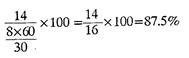
In time study based incentive schemes the bonus or the reward is related to a factor known as Operator Performance which is

Suppose there is 8 hour duty and a job should take 30 minutes to complete (standard performance), but after 8 hours an operator is able to complete only 14 such jobs. Therefore the operator performance is,

Example 5:

Given:

Base wage rate: Rs. 4/hour

Bonus at standard performance: 33.33%

Total items to complete: 50

Processing time for each item: 3 minutes.

Work completed in: 140 minutes.

To find: Bonus earned.

Solution:

Earning rate of the operator = Base wage rate per hour + (Bonus) (Wage rate)

= 4 + [(33.33)/100] 4 = Rs.5.33

Earning rate per minute = Rs.5.33/60 = Rs. 0.0888

Operator’s actual earnings

= (No. of items to be made) x (time for one item) x (earning rate)

= 50 x 3 x 0.08S8 = Rs. 13.32 …(1)

Operator’s earnings depending upon base wage rate

= (time taken to complete the work) x (Base wage rate)

= 140/60 (Hrs)x Rs. 4/hour = Rs. 9.33

Therefore the bonus (or reward) earned by the Operator

= (1) – (2)

= Rs. 13.32—Rs. 9.33

= Rs. 3.99 or Rs. 4.

Readers may try the following problem for the sake of practice.

Comparison of Work Measurement Techniques:

Technique # 7. Ergonomics:

Ergons means ‘Work’ and Nomos means ‘Natural Laws’. Ergonomics or its American equivalent ‘Human Engineering’ may be defined as the scientific study of the relationship between man and his working environments. Ergonomics implies ‘Fitting the job to the worker’. Ergonomics combines the knowledge of a psychologist, physiologist, anatomist, engineer, anthropologist and a biometrician.

Objectives:

The objective of the study of ergonomics is to optimize the integration of man and machine in order to increase work rate and accuracy.

It involves the design of:

(i) A work place befitting the needs and requirements of the worker,

(ii) Equipment, machinery and controls in such a manner so as to minimize mental and physical strain on the worker thereby increasing the efficiency, and

(iii) A conducive environment for executing the task most effectively.

Both Work study and Ergonomics are complementary and try to fit the job to the workers; however, Ergonomics adequately takes care of factors governing physical and mental strains.

Applications:

In practice, ergonomics has been applied to a number of areas as discussed below:

(i) Working environments,

(ii) The workplace, and

(iii) Other areas.

(i) Working Environments:

(a) The environment aspect includes considerations regarding light, climatic conditions (i.e., temperature, humidity and fresh air circulation), noise, bad odour, smoke, fumes, etc., which affect the health and efficiency of a worker.

(b) Day light should be reinforced with artificial lights, depending upon the nature of work.

(c) The environment should be well-ventilated and comfortable.

(d) Dust and fume collectors should preferably be attached with the equipment giving rise to them.

(e) Glares and reflections coming from glazed and polished surfaces should be avoided.

(f) For better perception, different parts or sub-systems of an equipment should be coloured suitably. Colours also add to the sense of pleasure.

(g) Excessive contrast, owing to colour or badly located windows, etc., should be eluded.

(h) Noise, no doubt distracts the attention (thoughts, mind) but if it is slow and continuous, workers become habituated to it. When the noise is high pitched, intermittent or sudden, it is more dangerous and needs to be dampened by isolating the place of noise and through the use of sound absorbing materials.

(ii) Work Place Layout:

The workplace is a space in a factory/machine which must accommodate an operator(s), who may be sitting or standing. Ideally, a workplace should be custom built for the use of one person whose dimensions are known. For general use, however, a compromise must be made to allow for the varying dimensions of humans. Therefore, a workplace should be so proportioned that it suits a chosen group of people.

Adjustment may be provided (on seat heights for example) to help the situation. Fig. 9.21 shows suggested critical dimensions for a group of males using a seated workplace. These dimensions can be obtained quickly and easily and will be quite satisfactory for construct­ing a mock-up of the proposed design.

The Fig. 9.21 shows the left hand covering the maximum working area and the right hand covering the normal working area. Normal working area is the space within which a seated or standing worker can reach and use tools, materials and equipment when his elbows fall naturally by the side of the body. Maximum working area is the space over which a seated or standing worker has to make full length arm movements (i.e., from the shoulder) in order to reach and use tools, materials and equipment.

Assuming the work as some operation requiring equipment, any tools, bins, etc., they should be placed within the area shaded so that they can be seen and reached quickly and easily. Fig. 9.22 shows the situation with respect to bench heights and seat heights. In this view, the seat should be adjustable for height and rake. It is not usually convenient to have adjustable benches or work tops and the value of 712mm to 762mm is probably the best compromise dimension.

Workplace layout, design of seat, arrangement of different equipment, tools and components should not cause discomfort to the worker. The seat should be such that the worker is able to adopt different postures, if necessary, for carrying out different operations. The height and back of the chair should be adjustable. A proper foot rest, arm rest and leg room should be provided. While working, an operator should feel himself natural and comfortable.

Design and layout of display panels and instrument dials should result in accurate observations. They should preferably form a part of the workplace and the display should be easily readable by all. Also the display panel should be at right angles to the line of sight of the operator. An instrument with a pointer should be employed for check readings whereas for quantitative readings, digital type of instruments should be preferred.

Design and location of various manual controls, knobs, wheels and levers should not cause excessive physical and mental strain to the worker. Levers and controls should be located close to the operator. Hand and foot controls, both, should be employed to advantage. All controls should preferably move in one direction for one kind of action. For example, upward movement of the levers should energise the subsystem and downward motion should de-energise and vice versa.

In the case of tote boxes, bins, loose or portable tools, etc., there should be a definite place for their location within the working area. Hence the operator can develop habitual, confident movements when reaching for equipment often without any need for the eyes to direct the hands. The mental effort and strain are less. For the same reason, material and tools used at the workplace should always be located within the working area to permit the best sequence of operations (refer Fig. 9.23).

The operation shown consists of assembling four parts A, B, C and D (two assemblies at a time) using both hands. As finished assemblies are placed in chutes, parts A are in the next bins as they are required first for the next assembly. Where possible, clear access should be given around industrial workplaces to allow for adequate supervision and inspection. It is clear that if ergonomic principles are observed in the design of workplaces, then the operator will be more efficient, less strained and tired and consequently less liable to have an accident.

(iii) Other Areas:

Other areas include studies related to fatigue, losses caused due to fatigue, rest pauses, amount of energy consumed, shift work and age considerations.