
The below mentioned article will help you to prepare a project report on Inventory Control and Management.
Inventory:
Inventory is a detailed list of those movable items which are necessary to manufacture a product and to maintain the equipment and machinery in good working order. The quantity and the value of every item is also mentioned in the list.
Inventory is actually ‘money’ kept in the store room in the shape of a high speed steel bit, a mild steel rod, milling cutters or welding electrodes.
Inventory Control:
Inventory control is concerned with achieving an optimum balance between two competing objectives.
ADVERTISEMENTS:
The objectives are:
(i) To minimize investment in inventory,
(ii) To maximize the service levels to the firm’s customers and its own operating departments.
Inventory control may be defined as the scientific method of finding out how much stock should be maintained in order to meet the production demands and be able to provide right type of material at right time in the right quantities and at competitive prices.
Inventory Classification:
ADVERTISEMENTS:
Inventory may be classified as follows:
(i) Raw inventories:
They include raw material and semi-finished products supplied by another firm and which are raw items for the present industry.
(ii) In-process inventories:
ADVERTISEMENTS:
They are semi-finished goods at various stages of manufacturing cycle.
(iii) Finished inventories:
They are the finished goods lying in stock rooms and waiting dispatch.
(iv) Indirect inventories:
ADVERTISEMENTS:
They include lubricants and other items (like spare parts) needed for proper operation, repair and maintenance during manufacturing cycle.
Inventory Management:
To manage these various kinds of inventories two alternative control procedures can be used:
(1) Order point system:
This has been the traditional approach to inventory control. In this system, the items are restocked when the inventory levels become low. Lot size and reorder point calculations are the more spectacular aspect of inventory management. Once the calculations are complete, the routing commences for checking deliveries and physical count of the amount on hand.
ADVERTISEMENTS:
(2) Materials requirements planning (MRP):
MRP is sometimes thought of as an inventory control procedure. It is really more than that. MRP is the technique used to plan and control manufacturing inventories. MRP is a computational technique that converts the master schedule for end products into a detailed schedule for the raw material and components used in the end products.
The detailed schedule identifies the quantities of each raw material and component item. It also tells when each item must be ordered and delivered so as to meet the master schedule for the final products.
It is important that the proper control procedure be applied to each of the four types of inventory as explained earlier.
ADVERTISEMENTS:
In general, MRP is appropriate control procedure for inventory type (i) and (ii) (i.e., raw materials, purchased components and in-process inventory).
Order point systems are often considered as the appropriate procedure to control inventory types (iii) and (iv) (i.e., finished goods, maintenance and repair parts, cutting tools and fixtures, plumbing supplies etc.).
Inventory Control, Its Objectives and How to Achieve Them:
Inventory control aims at keeping track of inventories. In other words, inventories of required quality and in desired quantities should be made available to different departments as and when they need.
This is achieved by:
ADVERTISEMENTS:
(a) Purchasing material at an economical price, at proper time and in sufficient quantities so as not to run short of them at any instant.
(b) Providing a suitable and secure storage location.
(c) Providing enough storage space.
(d) A definite inventory identification system.
(e) Adequate and responsible store room staff.
(f) Suitable requisition procedure.
ADVERTISEMENTS:
(g) Up-to-date and accurate record keeping.
(h) Periodic inventory checkup.
(i) Division of inventory under A, B and C items, exercising the control accordingly and removing obsolete inventory.
A good control over the inventories offers the following Advantages:
(a) One does not face shortage of materials.
(b) Materials of good quality and procured in time minimises defects in finished goods.
ADVERTISEMENTS:
(c) Delays in production schedules are avoided.
(d) Production targets are achieved.
(e) Accurate delivery dates can be ascertained and the industry builds up reputation and better relations with customers.
Functions of Inventories:
1. Separate different operations from one another and make them independent, so that each operation (starting from raw material to finished product) can be performed economically.
For example, ordering of raw material can be carried out independently of the finished goods distribution and both of these operations can be made low cost operations say by ordering raw material and distributing finished goods in one big lot, than in small batch sizes. Besides economy, the men and machinery also can be better utilized if the operations are separated and carried out in various departments than if coupled and tied at one place.
2. Maintain smooth and efficient production flow.
ADVERTISEMENTS:
3. Purchase in desired quantities and thus nullify the effects of changes in prices or supply.
4. Keep a process continually operating.
5. Create motivational effect. A person may be tempted to purchase more if inventories are displayed in bulk.
Economic Order Quantity:
A problem which always remains is that how much material may be ordered at a time. An industry making bolts will definitely like to know the length of steel bars to be purchased at any one time. This length of steel bars is called “Economic Order Quantity” and an economic order quantity is one which per units lowest cost per unit and is most advantageous.
Before calculating economic order quantity it is necessary to become familiar with terms like maximum inventory, minimum inventory, standard order and reorder point, which are known as Quantity Standards. Figure 24.1 shows different quantity standards.

Starting from an instant when inventory OA is in the stores, it (inventory) consumes gradually in quantity from A along AD at a uniform rate. It is pre-known that it takes L number of days between initiating order and receiving the required inventory.
ADVERTISEMENTS:
Therefore as the quantity reaches point B, purchase requisition is initiated which takes from B to C, that is time R. From C to D is the inventory procurement time P. At the point D when only reserve stock is left, the ordered material is supposed to reach and again the total quantity shoots to its maximum value, i.e. the point A'(A=A’).
Maximum Quantity OA is the upper or maximum limit to which the inventory can be kept in the stores at any time.
Minimum Quantity OE is the lower or minimum limit of the inventory which must be kept in the stores at any time.
The purpose should be to hold enough and not excessive stock of material.
Stock holding:
ADVERTISEMENTS:
(a) Avoids running out of stock.
(b) Helps creating a buffer stock which may be utilized if the material falls below the mini mum level.
(c) Makes sure the pre-decided delivery dates.
(d) Provides quick availability of materials.
(e) Takes care of price fluctuations and shortage of inventory in the market.
(f) Advises regarding, obsolete and slow moving items.
(g) Helps in standardization and thus reducing the variety of items to be handled.
Standard order:
(A’D) is the difference between maximum and minimum quantity and it is known as economical purchase inventory size.
Reorder Point (B) indicates that it is high time to initiate a purchase order and if not done so the inventory may exhaust, and even reserve stock utilized before the new material arrives.
From B1 to D1 it is as lead time (L) and it may be calculated on the basis of past experience.
It includes:
(a) Time to prepare purchase requisition and placing the order;
(b) Time taken to deliver purchase order to the seller;
(c) Time for seller (vendor) to get or prepare inventory; and
(d) Time for the inventory to be dispatched from the vendor’s end and to reach the customer.
Time, (a) above is known as requisition time (R) and (b) + (c) + (d) is the procurement time (P).
The economic lot size for an order or the economic order quantity depends upon two types of costs:
(a) Inventory procurement costs, which consist of expenditure connected with:
1. Receiving quotations;
2. Processing purchase requisition;
3. Following up and expediting purchase order;
4. Receiving material and then inspecting it; and
5. Processing seller’s (vendor’s) invoice.
Procurement costs decrease as the order quantity increases (see Fig. 24.2).
(b) Carrying costs, which vary with quantity ordered, base on average inventory and consist of:
1. Interest on capital investment;
2. Cost of storage facility, up-keep of material, record keeping etc.;
3. Cost involving deterioration and obsolescence; and
4. Cost of insurance, property tax, etc.
Carrying costs are almost directly proportional to the order size or lot size or order quantity.

In Fig. 24.2 the procurement costs and inventory carrying costs have been plotted with respect to quantity in lot. Total cost is calculated by adding procurement cost and carrying cost. Total cost is minimum at the point, A and thus A’ represents the economic order quantity or economic lot size.
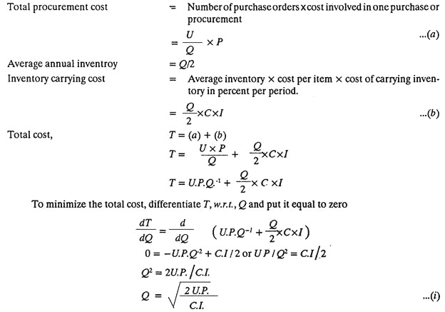
Another method of finding E.O.Q. that is by mathematical means, is given below:
Let Q is the economic lot size or E. O. Q.
C is the cost for one item.
I is the cost of carrying inventory in percentage per period, including insurance, obsolescence, taxes etc.
P is the procurement cost associated with one order,
and U is total quantity used per period say annually.
Number of purchase orders to be furnished
![]()
Example 1: Given that:
(i) Annual usage, U = 60 units
(ii) Procurement cost, P = Rs.15 per order
(iii) Cost per piece, C = Rs. 100
(iv) Cost of carrying inventory/, a percentage including expenditure on obsolescence, taxes, insurance, deterioration etc. = 10%. Calculate E.O. Q.
Solution:
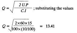
Therefore, number of order per year = 60/13.41 = 4.47 say 5.
Hence Q or E.O.Q = 12 units.
Inventory Models:
Inventory models determine when and how much inventory to carry.
Inventory models handle chiefly two decisions.
(1) How much to order at one time, and
(2) When to order this quantity to minimize total costs.
Lowest-cost decision rules for inventory management pertain to either buying products from outside or producing them within the company. Simple inventory models assume no delivery delay and that demand is known. Probabilistic models handle situations of risk and uncertainty.
Types of inventory models:
(1) Simple EOQ model:
a. The simple EOQ model can be used if the demand is known with certainty
b. The demand and lead time are known.
c. The item will be purchased from outside (the firm) and that demand will continue well into the future.
d. It is also assumed that not only the demand is known with certainty, but that is the same from day to day and that stock-outs, are not allowed. Under these assumptions, Fig 24.3 depicts the inventory position through time.

If we start to observe the inventory position immediately after receipt of an order, the quantity in stock Q decreases steadily until a lead time’s supply is reached. If lead time (L) is 5 days and demand is 4 (pieces) per day, a lead time’s supply is 20 pieces or units. Therefore when 20 units remain in the store, an order is placed. This is called the re-order point. Exactly 5 days after the order is placed, the stock is replenished and the cycle repeats itself.
(2) EOQ model with stock-out allowed:
Stock-out means running out of stock. In simple EOQ model, the stock was always available. The out of stock position will lead to a back order. This situation is frequently found in mailing- order houses where an item is temporarily out-of-stock and the customer is willing to wait until it is replenished.
The firm does suffer some cost in this situation, since, at the very least, some expediting and extra communication (perhaps in the form of telephone calls or postcards) with the customer, must take place. In addition to the explicit costs, repeated backorders will certainly lead to an erosion of goodwill. In some situations, backorders may be economically justified.
For instance, with very high-value items such as commercial jet planes, no inventory is carried and a backorder state always exists. The second possible outcome of an out-of stock position is the lost sales. Here the cost is much more severe. In this case, the customer places an order, receives an out-of-stock response, and takes his business elsewhere.
The company must take into account the likelihood that the customer will hot return and that therefore the profit on future sales might also be lost. In addition, the loss in goodwill that this will precipitate may also persuade others to purchase elsewhere. Since backorder and lost sales costs are hard to estimate, service levels are frequently specified. For example, management may feel that stock-outs should not occur more than 2% of the time.
Fig 24.4 shows time pattern of inventory levels when stock-outs are incurred.

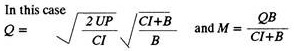
where Q is Economic order quantity
U is Annual use
P is Procurement cost per order
C is cost per piece
I is cost of carrying inventory, a percentage- including insurance, obsolescence, taxes etc.
B is cost incurred for every backorder
M is maximum inventory.
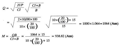
Example 2:
Find Q and M from the following data:
U = 10,000 units, P = Rs. 100 per order, C = Rs. 10 per unit
B = Rs. 15 per each backorder incurred, I = 20%
Solution:
(3) Inventory model under risk:
In the simple EOQ model it was assumed that demand and lead time were both known with certainty. Under this condition, whenever inventory levels reached a lead time’s worth of demand, an order was placed. Then as the stock was finally depleted, a replenishment order would arrive. We did find, however, that if backorders had a finite cost, a reorder level below the average lead time demand may be appropriate.
This strategy would result in some desired number of backorders. We can, therefore, conclude that the purpose of reorder levels is not to prevent stock-outs, but to keep them within desired limits. In the case of fluctuating demand, it may be quite logical to set reorder levels above the average lead time demand; for if we reorder when there is only enough in stock to meet the average demand during lead time, an out-of stock position will occur whenever demand exceeds this average value.
To protect from undesirably large stock-out situations, safety stocks (reserves) are maintained. They will provide the cushion needed whenever demand exceeds this average. Safety stocks (OS) can be defined as the difference between the reorder level and the average lead time demand (Fig. 24.5) Therefore as the reorder point is raised, the safety stock increases and the likelihood of a stock-out during any cycle decreases.

Fig. 24.5 shows the inventory pattern through time for a particular item which exhibits fluctuating demand. An order is placed whenever stock levels fall to Y. On the average, stock will be depleted to ‘s’ when the replenishment order arrives. During the first cycle we see that demand was about average; however in the second cycle (Fig. 24.5) the demand was much greater than average.
Protecting the system from a stock-out during the lead time was a safety stock maintained at S. If more protection was desired, the level of ‘r’ could have been increased. With a higher ‘r’, the safety stock would have been larger and the chances of a stock-out occurring in any one cycle would have been lower. Table 24.1, was compiled from data collected over several periods.
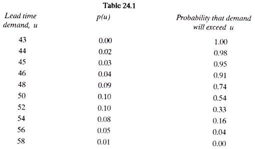
When P (u) = 0.02, it implies that for 2% of these periods demand was 44, in 3% of them, demand was 45 and so on.
The last column in Table 24.1 illustrates the probability that demand will exceed any of these levels, u. For example, the probability that demand will exceed 56 units is 0 04. The last column will be very useful for setting safety stocks when a service criterion is given.
In many cases, it might be quite difficult to determine the actual cost of a stock-out. An indirect way to assess this is to specify a service level. For example, the manager of the product line whose lead time was recorded in Table 24.1 might feel that the likelihood of a stock-out should not exceed 4% during any one cycle. Therefore, the reorder point should be set at r = 56. We would, therefore, expect an out,-of-stock situation to occur in only one out of 25 ordering periods.
ABC Analysis:
Necessity:
As the size of the industry increases, the number of items to be purchased and then to be taken care of also increases. Purchase and control of all items at a time and in bulk much before their use, irrespective of their usage value, price or procurement problems, blocks and involves a lot of money and man hours, and is therefore uneconomical.
ABC analysis helps segregating the items from one another and tells how much valued the item is and controlling it to what extent is in the interest of the organisation.
Procedural steps:
1. Identify all the items used in an industry.
2. List all the items as per their value.
3. Count the number of high valued, medium valued and low valued items.
4. Find the percentage of high, medium and low valued items. High valued items normally contribute for 70% or so of the total inventory cost and medium and low valued items, 20 and 10% respectively.
5. A graph can be plotted between percent of items (on x-axis) and per cent of total inventory cost (on y-axis). Figure 24.6 shows such a graph.
It can be seen that 70% of the total inventory cost is against 10% of the total items (called A-items), 20% against 20% of the items (B-items) and 10% against a big bulk, i.e. 70% of the items (called C-items).
Thus ABC analysis furnishes the following information:
1. A-items are high valued but are limited or few in number. They need careful and close inventory control. Minimum and maximum limits, and reorder point is set for A items. Such items should be thought of in advance and purchased well in time. A detailed record of their receipt and issues should be kept, and proper handling and storage facilities should be provided for them.
Such items being costly are purchased in small quantities often and just before their use. This of-course increases the procurement costs and involves a little risk of non-availability. However, the locked up inventory cost decreases and the problems of storage and care taking are minimized.
A-items generally account for 70-80% of the total inventory cost and they constitute about 10% of the total items.

2. B-items are medium valued and their number lies in between A and C-items. Such items need moderate control. They are more important than C-items. They are purchased on the basis of past requirements, a record of receipts and issues is kept and a procurement order is placed as soon as the quantity touches reorder point. These items being comparatively less costly, a safety stock of up to 3 months may be kept, whereas it needs a stock of fortnight or so in case of A items. 5-items also require careful storage and handling.
In brief, 5-items need every care but not so intensive as is required for A -items.
B-items generally account for 20 to 15% of the total inventory cost and constitute about 15 to 20 % of the total items.
3. C-items are low valued, but maximum numbered items.
These items do not need any control, rather controlling them is uneconomical. These are the least important items like clips, all pins, washers, rubber bands, etc. They are generally procured just before they finish. No expediting is necessary, no records are normally kept and a safety stock of 3 months or even more can be purchased at an instant. Future requirements of such items are never calculated and a two bin system is sufficient to hint procurement.
C-items generally account for 10 to 5% of the total inventory cost and they constitute about 75% of the total items.
Material Requirements Planning (MRP):
MRP is a computational technique that converts the master schedule for end products into a detailed schedule for raw material and components used in the end products. The detailed schedule identifies the quantities of each raw material and component items. It also tells when each item must be ordered and delivered so as to meet the master schedule for the final products.
The purpose of MRP is to ensure that materials and components are available in the right quantities and at the right time so that finished products can be completed according to the master production schedule. MRP is often considered to be a subset of inventory control. It is an effective tool for minimizing unnecessary inventory investment.
MRP is also useful in production scheduling and purchasing of materials. The concept of MRP is relatively straight forward. What complicates the application of the technique is the sheer magnitude of the data to be processed.

Functions:
An MRP system has three major Functions /uses:
1. Control of inventory levels,
2. Assignment of priorities for components, (depending upon their delivery dates) and
3. Determination of capacity requirements at a detailed level.
Capacity requirements planning (CRP) is a system for determining if a planned production schedule can be accomplished with available capacity and, if not, making adjustments as necessary.
Inputs to MRP:
MRP converts the master production schedule into the detailed schedule for raw materials and components. For the MRP program to perform its function, it must operate on the data contained in the master schedule. However, this is only one of three sources of input data on which MRP relies.
The three inputs to MRP are:
1. The master production schedule and other order data.
2. The bill-of-material file, which defines the product structure.
3. The inventory record file.
Fig 24.8 shows the flow of data into the MRP processor and its conversion into useful output reports.

Master production schedule:
The master schedule is based on an accurate estimate of demand for the firm’s product, together with a realistic assessment of its production capacity. The master production schedule (Fig. 24.9) is a list of what end products are to be produced, how many of each product is to be produced, and when the products are likely to be ready for shipment.

The general format of a master production schedule is illustrated in Fig 24.9. It may show weekly or monthly delivery schedules.
Bill-of-materials file:
In order to compute the raw material and component requirements for end products listed in the master schedule, the product structure must be known. This is specified by the bill-of-materials which is a list of component parts and sub-assemblies that make up each product. Putting all these assembly lists together, we have the bill-of-materials file (BOM). Fig 24.10 shows the structure of an assembled product. It shows, subassembly S1 is the Parent of components C1 C2 and C3 Product P1 is the parent of sub-assemblies S1 and S2 and so on.

The product structure must also specify how many of each item are included in its parent. This is accomplished in Fig. 24.10 by the number in parentheses to the right and below each block. For example, subassembly S1 contains four of components C2 and one each of components C1 and C3.
Inventory record file:
It is mandatory in MRP to have accurate current data on inventory status. This is accomplished by utilising a computerized inventory system which maintains the inventory record file or item master file. (Fig. 24.11).

A definition of the lead time for the raw material, components and assemblies must be established in the inventory record file. The ordering lead time can be determined from purchasing records. The manufacturing lead time can be determined from the process route sheets.
It is important that the inputs to the MRP processor be kept current. The bill-of-materials file must be maintained by feeding any engineering changes that affect the product structure into the BOM. Similarly, the inventory record file is maintained by inputting the inventory transactions to the file.
Working of MRP:
The MPR processor (Fig 24.8) operates on data contained in the master schedule, the bill-of- materials file and the inventory record file. The master schedule specifies a period-by-period list of final products required. The BOM defines what materials and components are needed for each product. The inventory record file contains information on the current and future inventory status of each component.
The MRP program computer-how many of each component and raw material are needed by exploding the end product requirements into successively lower levels in the product structure. Referring to master schedule (Fig 24.9), 50 units of product P1 explode into 50 units of subassembly S, and 100 units of S2 and components: C1 = 50, C2 = 200, C3 = 50, C4 = 200, C5 = 200 and C6 = 100 units. The quantities of raw materials for these components would be determined in a similar manner.
There are several factors that must be considered in the MRP parts and materials explosion.
They are:
(1) Components and subassemblies already existing in the stock must be considered for determining requirements for meeting the master schedule.
(2) The MRP processor must determine when to start assembling the subassemblies by offsetting the due dates for these items by their respective manufacturing lead times. Similarly, the component due dates must be offset by their manufacturing lead times.
The MRP program performs these lead-time-offset calculations from data obtained in the inventory record file and from route-sheet data.
(3) Some components and many raw materials are common to several products. The MRP processor must collect these common use items during the part explosion. The total quantities for each common use item are then combined into a single net requirement for the item.
(4) Since blaster production schedule provides time-phased delivery requirements for the end products, this time phasing must be carried through the calculations of the individual component and raw material requirements.
MRP Output reports:
The MRP program generates a variety of outputs that can be used in the planning and management of plant operations.
These outputs include:
(a) Primary outputs:
(1) Order release notice, to place orders that have been planned by the MRP system.
(2) Reports showing planned orders to be released in future periods.
(3) Rescheduling notices, indicating changes in due dates for open orders.
(4) Cancellation notices, indicating cancellation of open orders because of changes in the master schedule.
(5) Reports on inventory status.
(b) Secondary outputs:
(1) Performance reports of various types, indicating costs, item usage, actual versus planned lead times etc.
(2) Exception reports, showing deviations from schedule, orders that are overdue, scrap and so on.
(3) Inventory forecasts, indicating projected inventory levels in future periods.
Benefits of MRP:
(1) Reduction in inventory.
(2) Improved customer service-late orders are reduced as much as 90%.
(3) Quicker response to changes in demand.
(4) Better machine utilization.
(5) Greater productivity.
Manufacturing Resource Planning (MRP II):
MRP was originally developed as a computer system for planning material orders. Manufacturing personnel soon discovered that capacity planning and scheduling could be integrated with MRP and the closed loop MRP concept was born. More sophisticated software packages evolved into complete manufacturing control systems. The use of an MRP-based system to plan all the resources of a manufacturing company is called MRP II.
MRP II includes strategic financial planning as well as production planning through the use of simulation capabilities to answer what-if questions. What-if capabilities are routinely used to evaluate alternative plans. MRP II is a total company system, in which functional groups interact commonly and formally and make joint decisions. Finally, the system is user-transparent.
Users at all levels understand and accept the logic and realism of the system and need not work outside the formal system. Fig 24.12 shows one such system – MRPS. Manufacturing Resource Planning System developed by CINCOM systems, Inc. MRPS includes the vertical dimension of production planning, master production scheduling, MRP and shop floor control. The system also expands horizontally to include inventory control, purchasing and other planning considerations.

Operating Cycle:
The operating cycle refers to the length of time necessary to complete the following cycle of evens’:
1. Convert cash into inventory.
2. Convert inventory into receivables.
3. Convert receivable into cash.
In phase 1, cash is used to produce inventory. For manufacturing firms, this phase would start with the purchase of raw materials and would conclude with the manufacturing process delivering goods to inventory. In the second phase of the cycle the inventory is converted into receivables as sales are made to customers.

The last phase of the operating cycle, phase 3, sees the receivables being collected and the operating cycle is complete.
Firms that have no credit terms (cash and carry firms) would have no phase 2 since they will sell only on cash. Receivables are notes and acceptances receivables. These are short term promissory instruments of indebtedness that reflect obligations owed the firm.