Cost Types: 8 Main Types of Costs

Since there are large number of determinants which influence the cost. These determinants vary from situation to situation, and enterprise to enterprise. Therefore for taking a decision about any such determinants, we must analyse them thoroughly. In order to take write deci­sions, it is necessary to understand different costs.

Some of them are explained hereunder:

1. Actual Costs:

These are the costs which the firm incurs while producing or acquiring a good or a service. The actual costs are also known as acquisition cost or outlay costs. The ex­amples of such costs are material costs, labour costs, rent etc.

2. Opportunity Cost:

Opportunity cost represents the benefits or revenue forgone by pur­suing one course of action rather than other. This means, when best alternative is adopted, it is obvious that second best alternative cannot be implemented and its benefits are forgone.

Thus the benefit of this second best alternative which has been sacrificed due to the selection of best alternative is known as the opportunity cost of the best alternative.

Opportunity costs can also be defined as, the return from the second best use of the firm’s resources which the firm forgoes in order to avail of the return from the best use of the re­sources.

Some examples of opportunity cost are:

(a) Opportunity cost of the funds employed in the firm is the amount of interest which otherwise could have been earned.

(b) Opportunity cost of labour in own business is the income which he would have earned by accepting a job outside.

(c) Opportunity cost of space used in expansion of the business is the amount of rent which could be fetched if it is rented out to somebody else.

3. Marginal Cost:

Marginal cost is the increase in cost as a result a unit change in output.

Marginal cost can also be defined as, the additional costs incurred when there is a unit change in the existing output of goods and services.

In mathematical term, marginal cost of n^th unit M. C_n is the difference between the total cost of n^th unit T. C_n and the total cost of (n – 1)^th unit (T. C_n-1)

MC_n = TC_n – TC_n-1

In other words, marginal cost is the rate at which total cost changes with the change in output.

4. Incremental Costs:

Incremental costs may be defined as:

(а) The difference in total costs resulting from a contemplated change in policy or

(b) The addition to costs resulting from a change in the nature and the level of business activity.

The examples of the change are change in output level, product line, or product mix; adding or replacing a machine or distribution channel; advertising policy or level of investment.

While taking a decision, it may be ascertained that incremental revenue should exceed incremental cost. Incremental revenue is a change in total revenue resulting from a change. The difference between incremental revenue and incremental cost is known as incremental income.

5. Sunk Costs:

Sunk costs are the costs that are not altered by a change in quantity and cannot be recovered e.g., depreciation. This may also be defined as the cost for which the expen­diture has been incurred in the past and which will not be affected by the particular decision. These are the parts of the outlay (actual) costs.

6. Fixed and Variable Costs:

Fixed costs are the part of the total cost of the firm which do not vary with the variation in the output. Examples of the fixed costs are rent of land or build­ing, property tax etc. The fixed cost are also known as overhead costs or indirect costs. If the production increases the fixed cost per unit decreases, as the total fixed cost is divided between large number of units.

Variable costs, are directly dependent on the volume of production or service. Examples of variable costs are material costs, labour costs etc.

7. Short Run and Long Run Costs:

To understand short run cost and long run cost, we must first discuss ‘short run’ and ‘long run’. Short run is a period in which the firm is free to vary its output but does not have the time to change its scale of plant. As inputs, like machin­ery, buildings etc., cannot be changed by the firm at any moment, since it takes time to replace, add or dismantle them.

To meet increased demand, in such circumstances, only way is to in­crease output by intensive working of existing capital equipment. Whereas if demand decreases, the output can be reduced by keeping equipment idle for proportionate period of time.

Long run is a period in which all inputs can be varied as desired. This is a period long enough to enable to adjust its supply and output completely to changes in demand.

Short run costs are the costs that vary with the degree of plant utilisation (i.e., output) and other fixed factors. It is the short run while fixed costs remain unchanged, variable costs fluctu­ate with the output.

Long run costs, on the other hand, are the costs that vary with the size of plant. ‘Short run’ and ‘long run’ costs are used for predicting the effect of temporary, and permanent output decisions on costs, prices, and hence profits.

8. Cost-Output Relationship:

Cost-output relationship for short and long described here­under:

(A) For Short Run:

For short run, the total Cost (TC) to a firm for a given level of output is the sum of the total variable cost (TVC) and the total fixed cost (TFC).

TC = TFC + TVC

These, average costs can be represented, graphically as shown below:

The properties of average cost curves are:

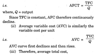
(i) AFC declines continuously, approaching both axes asymptotically.

(ii) AVC first declines, reaches a minimum, and then rises.

(iii) When AFC approaches asymptotically the horizontal axis, AVC approaches ATC as­ymptotically.

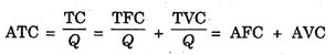
(iv) ATC first declines, reaches a minimum, and then rises. When it is minimum, output is at optimum level.

B. For Long Run:

As already discussed under heading ‘long run costs’, in the long run, all factors are variable and the firm has number of alternatives. For example, a firm has two choices for production i.e., small or medium size plant. These plants operate with average costs of AC₁ and AC₂ respectively.

Here, for production between Q₁ and Q₂ only one option i.e. with small plant, is available, whereas for production between Q₂ and Q₃ both the options i.e., either to use small plant or medium size plant are available. Again for production between Q₃ and Q₄ only medium size plant can be used. These curves help to find out which option is economical for a particular level of output.

Here we have discussed only two options, but in practice large number of options is avail­able. In such circumstances curves can be drawn for each alternative and then best is selected for a particular level of output.