Valuation of Put Option using Black-Scholes Model | Forex Management

An alternative form of valuation is to use the Black-Scholes formula for a put, which is:

P = Xe ^–r(T-t) [1-N(d₂)] – S [1-N(d₁)]

Where d₁ and d₂ are as given in the section deriving a call option.

Note that [1 – N(d₂)] is the same as N(-d₂) and [1 – N(d₁)] is the same as N(-d₁).

Using the same data that we used in valuing the call, the put option value is calculated as follows:

p = 31.6693(0.3446) – 35(0.2743) = 1.3127

Values for d₁ and d₂ must be computed first, and then a table for the standard normal distribution must be used to look up the N values. In actual practice, computer algorithms and handheld calculators use a polynomial equation that will give very accurate N value approximations.

As a matter of fact our standard procedure to value any asset consists of two basic steps:

(1) Forecasting expected cash flow and

(2) Discounting at the opportunity cost of capital.

This approach is not helpful for option valuation. In case of option, the first step is very complicated but feasible.

Finding the opportunity cost of capital is impossible because the risk of an option changes every time the stock price moves. It also changes over time even with the stock price constant. The trick in pricing any option is to set up a package of investment in the stock and a loan that will exactly replicate the payoffs from the option. Over the years a number of mathematical formulae have been evolved for calculating the value of an option.

The most important of these is the Black and Scholes Option Pricing Model (BSOPM). This model gives a formula by which the premium can be worked out. BSOPM has also served as foundation for further research into option pricing.

The BSOPM has proved flexible; it can be adapted to value options on a variety of assets with special features such as foreign currency bonds, and futures. It is an unpleasant-looking formula, but with the help of specially programmed calculator or a computer, one can easily compute option prices within seconds.

Although the formula appears quite forbidding using it is fairly direct.

The major inputs are:

(1) Current stock price ‘S’

(2) Exercise price ‘E’,

(3) Time to maturity ‘t’,

(4) Market interest rate ‘r’ and

(5) Standard deviation of annual price changes ‘s’.

The first three inputs are readily observable from current market quotations or are known items of data. The market interest rate must be estimated but it can be established fairly easily. Possible sources are the T-bill rate quoted daily for different maturities ranging from 30, 60 and 90 to 240 days. The rate for the maturity that corresponds to the term of the option should be used.

The other estimated input – the standard deviation of the stock price change – is more difficult to estimate and errors can have a significant impact on the established option value. There are several techniques for estimating the variability of the stock price. One technique uses historically derived values of the standard deviation of price changes of the stock as an estimate of the standard deviation to be generated in the future.

The time period of the measurements becomes important in this regard; too long a period may result in the inclusion of irrelevant observations and too short a period may exclude valuable information and not be representative. Some recommend the most recent six months’ or year’s trading data as the best measurement interval with the use of historical data.

An alternative way to estimate the variability of a stock is the option valuation formula. Rather than using the formula to assess the proper price of an option, we can observe the current price of an option and deduce the standard deviation of the stock price as implied in the formula.

Calculating and averaging the implied deviation over a series of past periods may provide a more accurate assessment of the expected variability of the stock than a straightfor­ward averaging of past values. In either case, it may be necessary to adjust these derived values for possible future changes in the variability of the stock price.

Here, we would want to examine those underlying factors that are basic determinants of the riskiness of securities:

(1) Interest rate risk,

(2) Purchasing power risk,

(3) Business risk and

(4) Financial risk.

If the exposure of the stock to these factors is changing, the historically derived variability estimate should be adjusted to reflect this change. For example, if the company is now financing more heavily with debt, its exposure to financial risk and expected future variability would be greater than in the past.

Problem 1:

The stock option have 120 days until expiration and the strike price is Rs.85. The simple rate of interest is 6 per cent p.a. The underlying asset value is Rs.80 and the volatility (standard deviation) is 0.30. Calculate the value of the stock option.

Solution:

(1) The number of days to expiration must be converted into years by dividing by 365

Thus, t = 120/365 = 0.329

(2) The simple annual interest must be converted to the Black – Scholes continuously compounded equivalent using the relationship that 1+R = e^r, making r = In (1+R).

Now r = In (1.06) = 0.0583

Now we can find the values of d₁ and d₂ as follows:

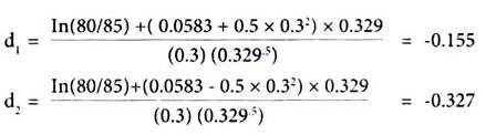
The next step is to look up the N(d₁) and N(d₂) values in a table of such Values. Note that N(d₁) = N (-0.155) and N(d₂) = (-0.327) represent areas under a standard normal distribution function. From Table given at the end of the book, we see that the value of d₁ = 0.155 implies the area under the normal curve to the left of -0.155, which is approximately (interpolating from the table) .438.

The value of N(d₂) is found in a similar fashion to be approximately 0.372.

Now, we can insert the above values in Black – Scholes formula, to obtain the value of the stock option.

= 80 x .438 x e^{(-0.0583 x .329)} x .372 = Rs.4.03

Problem 2:

Calculate the value of option from the following information:

S = Rs.20

r = 12% = 0.12

K = Rs.20

σ² = 0.16

t =3 months or 0.25 years

Solution:

Since d₁ and d₂ are required inputs for Black-Scholes Option Pricing Model.

 

d₂ = d₁ – 0.20 = 0.05

N(d₁) = N (0.25)

N(d₂) = N(0.052)

The above two represent area under a standard normal distribution function.

From table given at the end of the book, we see that value d₁ = 0.25 implies a probability of 0.0987 + 0.5000 = 0.5987, so N(d₁) = 0.5987. Similarly, N(d₂) = 0.5199. We can use those values to solve the equation in Black-Scholes Option Pricing Model.

C = Rs.20[N(d₁)] – Rs.20 e(-0.12)(0.25) [N(d₂)] = RS.20 [N(0.25)] – RS.20(0.9704)[N(0.05)]

= Rs.20(0.5987) – Rs. 19.41 (0.5199) = Rs. 11.97 – Rs.10.09 = Rs.1.88