This article throws light upon the top four methods of measurement of risk. The methods are: 1. Range Analysis 2. Probability Distribution 3. Standard Deviation 4. Coefficient of Variation.
Method # 1. Range Analysis:
Where different returns from an asset are possible under different circumstances, more than one forecast of the future returns may be made. These returns may be regarded as ‘optimistic’, ‘most likely’ and ‘pessimistic’.
The range of the returns is the difference between the highest possible rate of return and the lowest possible rate of return. According to this measure, an asset having greater range is said to be more risky than the one having lesser range. The following example illustrates the sensitivity analysis.
Example 1:
We can say that Asset B having greater range of returns is more risky.
Method # 2. Probability Distribution:
The risk associated with an asset can be measured more accurately by the use of probability distribution than the range analysis as the range is based on only two extreme values. The probability of an event represents the chances of its occurrence. For instance, if the chance of an event taking place is 3 out of 5, it can be said to have 60% chance or 0.60 probabilities.
While assigning probability, the following rules should be kept in mind:
(i) The possible outcomes must be mutually exclusive and collectively exhaustive,
ADVERTISEMENTS:
(ii) The probability assigned to an outcome may very between 0 and 1.
(iii) The sum total of probabilities must be equal to 1.
(iv) If an outcome is certain to occur, it is assigned a possibility of 1, while an impossible outcome is assigned a probability of 0. Thus, a probability can never be greater than 1 or lower than 0, it can never be a negative number.
The expected rate of return for any asset is the weighted average of all possible returns multiplied by their respective probabilities.
ADVERTISEMENTS:
This can be represented as below:
Where, E (R) = Expected return
n = Number of possible outcomes
ADVERTISEMENTS:
Pi = Possibility associated with ith possible outcome.
Ri = Rate of return for the ith possible outcome.
The expected rate of return for assets A and B is presented in the following example.
Example 2:
Method # 3. Standard Deviation:
Standard deviation is the most common quantitative measure of risk of an asset. Unlike the range, it considers every possible event and weight equal to its probability is assigned to each event. Standard deviation is a measure of dispersion around the expected or average mean value.
In this method the deviations are squared making all values positive. Then the weighted average of these figures is taken, using probabilities on weights. The result is termed as variance. It is converted to the original units by taking the square root. The result is termed as standard deviation. Symbolically,
where, s = Standard deviation
ADVERTISEMENTS:
n = Number of possible outcomes
Ri = Rate of return from the ith possible outcomes
E(R) = Expected return
Pi = Possibility associated with the ith possible outcome
ADVERTISEMENTS:
The greater the standard deviation of returns of an asset, the greater is the risk of the asset. Thus, the investor usually prefers investments with higher rate of return and lower standard deviation.
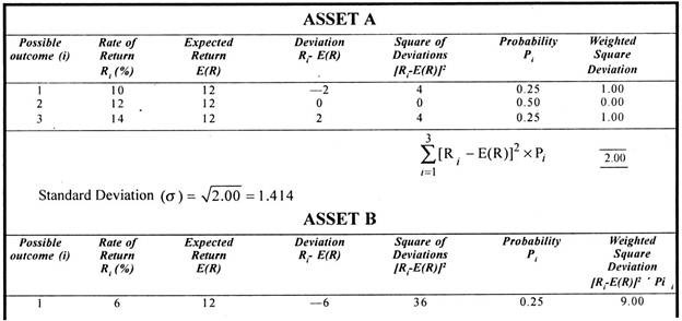
The following example illustrates the standard deviation measure of risk:
Example 3:
It is clear from the above that Asset B is more risky as the standard deviation of asset is greater than that of Asset B.
Method # 4. Coefficient of Variation:
ADVERTISEMENTS:
Standard deviation is an absolute measure of dispersion and it may give misleading results if the alternative assets differ in size of expected returns. In such a case, coefficient of variation may be used as a better measure of risk.
Coefficient of variation is a relative measure of dispersion in which risk per unit of expected return is calculated as below:
Coefficient of Variation = Standard Deviation/Mean
or, CV = σ/E (R)
Example 4:
The coefficient of variations for assets A and B are calculated as below:
ADVERTISEMENTS:
Coefficient of variation (Asset A) = 1.414/12 = 0.1178
Coefficient of variation (Asset B) = 4.243/12 = 0.3536
As the coefficient of variation of asset B is more, it can be said to be more risky as compared to asset A.


