
Here is an essay on ‘Linear Programming’ for class 11 and 12. Find paragraphs, long and short essays on ‘Linear Programming’ especially written for school and college students.
Essay on Linear Programming
Essay Contents:
- Essay on the Meaning of Linear Programming
- Essay on the Essential Ingredients of Linear Programming
- Essay on the Assumptions of Linear Programming
- Essay on the Uses and Applications of Linear Programming
- Essay on the Limitations of Linear Programming
- Essay on the Duality in Linear programming
Essay # 1. Meaning of Linear Programming:
Linear Programming is the analysis of problems in which a linear function of a number of variables is to be optimized when these variables are subject to a number of restraints in the form of inequalities. Linear programming helps the management to know either the maximum profit strategy or the best production programmes open to it.
ADVERTISEMENTS:
It is one of the most important tools of Operation Research used in management problems. Thus linear programming is a technique of selecting the best possible strategy from a number of alternatives. The chosen strategy is optimal in terms of maximization or minimisation of some desired action e.g. maximization of output or minimisation of production costs.
Linear programming from economist and businessmen viewpoint emerges due to scarce resources among alternative ends e.g. scarce resources for a firm are capital, personnel, equipment, material, warehousing etc.
Essay # 2. Essential Ingredients of Linear Programming:
Formulation of suitable mathematical model to explain the given situation is the starting point of linear programming.
The model can be conveniently framed by getting the answer to the following queries:
ADVERTISEMENTS:
(i) What factors or values are not known?
(ii) What is the objective?
(iii) What are the restrictions, specifications or constraints?
This information is then translated into the following ingredients of Linear Programming:
(a) Objective Function:
ADVERTISEMENTS:
The function to be optimized is known as objective function. It is some sort of linear mathematical relationship between the variables/factors under consideration. If the important features of a system can be explained by m factors X1 X2, …, Xm, then the objective function can be expressed in the linear form
Z = a1X1 + a2X2 +…+ amXm …(14.1)
where a1, a2,…, am are some known constants, generally known as prices associated with the variables. The objective function is always non-negative.
(b) Constraints or Linear Restrictions:
These are the set of restrictions imposed on the variables or some combination of few or all the variables appearing in the objective function. These constraints or restrictions are due to limitations of manpower, capacity of plant, capital available, time restrictions etc. i.e. the resources.
ADVERTISEMENTS:
These restrictions are never known in exact terms but are always given in some approximate terms i.e. less than or more than some given amount. In case it is known exactly, one can use well-known techniques of maxima and minima to find the optimum solution. But in practice the constraints are some algebraic inequalities expressed as ‘greater than (>); ‘less than (<)’, ‘greater than or equal to (≥)’ or ‘less than equal to (≤)’
e.g. b1X1 + b2X2 ≤ c
where b1, b2 and c are some constants,
The resource constraints are also assumed to be linear e.g. in a product mix l.p.p. it is assumed that each extra unit to be made requires exactly the same time as the previous unit. The inequalities i.e. the constraints in a problem can be more than one. All variables should have positive values.
(c) Feasible Solution:
ADVERTISEMENTS:
A feasible solution of a linear programming problem is a set of values for the variables X1, X2…., Xm which simultaneously satisfies all the constraints. For a given problem there can be many feasible solutions depending on the nature of the phenomenon.
Infeasible solution occurs to an I.p.p. if at least two of the constraints are conflicting in nature e.g. X1 + X2 ≥ 7 and X1 + X2 ≤ 1.
(d) Optimal Solution:
A feasible solution, which optimizes the objective function, is known as Optimal Solution. An optimal solution is always feasible but all feasible solutions cannot be optimal.
Essay # 3. Assumptions in Linear Programming:
The following assumptions may be true or valid over the area of search appropriate to the problem:
ADVERTISEMENTS:
(i) There are a number of restrictions or constraints expressible in quantitative terms.
(ii) The parameters are subject to variation in magnitude.
(iii) The relationships expressed by constraints and the objective functions are linear.
(iv) The objective function is to be optimized w.r.t. the variables involved in the phenomenon.
ADVERTISEMENTS:
The fundamental characteristic in all such cases is to find some optimum strategy under certain known specifications.
Essay # 4. Uses and Applications of Linear Programming:
Linear Programming supplies valuable information for proper planning and control of operations by evaluating an optimum combination of several factors (variables) involved in the phenomenon under known constraints e.g.
(i) Optimal Product Lines and Production Processes:
While operating at a high output level, a firm is likely to run into a variety of capacity limitations e.g. size of factory, amount of time available on different machines, warehouse space, skilled personnel.
All these may create bottlenecks. A crucial characteristic of such situation is that the production of a relatively unprofitable item or the use of a production process, which makes liberal use of the scarce facility may consume valuable capacity that could be otherwise used in more economical processes.
In other words an economy has at its disposal given quantities of various factors of production and a number of tasks to which these factors can be devoted. These factors can be allocated to different tasks in a number of different ways and one is interested in ‘best’ allocation.
Linear Programming gives solution to such situations providing a clear and sound understanding of the complex phenomenon to the executive by formulating:
ADVERTISEMENTS:
(i) The objectives to be pursued,
(ii) The various restrictions present,
(iii) The various alternative courses of actions and relationship between them, if any and
(iv) The contribution of each alternative action towards the accomplishment of the objectives.
The technique is based on some mathematical model building of the phenomenon and its analysis provides trustworthy interpretations.
The problems which can be effectively solved by linear programming techniques can be listed as:
ADVERTISEMENTS:
(i) Transport and Routing operations in the fields of agriculture, industry and military.
(ii) Production scheduling and inventory control.
(iii) Blending problems.
(iv) Least cost combination of inputs.
(v) Minimisation of raw materials waste.
(vi) Animal feed problem.
ADVERTISEMENTS:
(vii) Job assignment to Specialised personnel.
The fundamental characteristic in all such cases is to find some optimum strategy under certain known specifications.
Essay # 5. Limitations of Linear Programming:
(i) The assumption that all relations are linear may not hold good in many real situations e.g. production cost may not be a linear function of output; in the case of variable costs the profit coefficients may not satisfy the linearity restriction.
(ii) In L.P. all coefficients and constraints are stated with certainty.
(iii) The solution many times is in fractions, which may not remain optimal in rounding-off.
(iv) When the number of variables or constraints involved in the phenomenon is quite large then it may become necessary to use computers.
Essay # 6. Duality in Linear Programming:
It is observed that with every linear programming problem (known as Primal) there is always associated its Dual. The primal and the dual can be derived from each other and there is an unique dual associated with primal and vice-versa.
ADVERTISEMENTS:
The dual is obtained by transposing the rows and columns of the constraint, as well as transposing the co-efficient of the objective function and the right hand side values of the constraints. The inequalities are reversed and Maximisation problem (Minimisation problem) becomes Minimisation problem (maximisation problem).
It is observed that for every maximisation/minimisation l.p.p there is associated an unique minimisation/maximisation l.p.p based on the same information. The numerical values of the objective function in both cases remains same. Original problem is known as Primal and the associated problem as Dual. The dual can be derived from primal and vice-versa. The dual of the problem helps in investigating the effect to changes in the value of parameters of the problem.
Here all the constraints of primal in minimisation problem should be in ≤ form. In case some constraints are in ≥ or = form, then these should be converted in ≤ form by algebraic operations e.g.
Case (I):
a1 x1 + a2 x2 ≥ k1
ADVERTISEMENTS:
Can be written as
– (a1 x1 + a2 x2) ≤ – k1 (Multiplying both sides by- and reversing the inequality).
Similarly for a1 x1 + a2 x2 ≤ k1
We can write
Case (II):
This can be written as
a1 x1 + a2 x2 ≤ k1
a1 x1 + a2 x2 ≥ k1
one equality is converted in two inequalities
Now in case of maximisation Problem B is covered into ≤ type and for minimisation case A is changed into ≥ type by the method described in case (i).
In case of equality constraint one additional inequality is introduced in Primal.
If Primal is
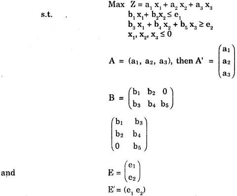
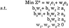
Since there are two constraint inequalities, the dual of the problem shall have two variables say w1 and w2. Now the dual of the problem will be
The following points should be noted:
(i) The parameters of Primal become the right hand side values of the constraints in Dual and the right hand side values of the constraints in Primal become the parameters of the Dual.
(ii) The number of variables Dual is equal to number of inequalities in Primal.
(iii) The matrix of the co-efficient of variables in left hand side of the constraints of Primal is transposed to get the matrix of co-efficient in L.H.S of the constraints in Dual.
(iv) The sign of inequalities of Primal are reversed in Dual.
(v) The dual of the dual is the primal problem.
The method is illustrated by the following example:
Example : Obtain the Dual of
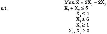
Here one constraint is X2 ≥ 1 which should be first changed in ≤ form as it is a maximisation problem. We get
– X2 ≥ – 1
The primal in matrix from will be
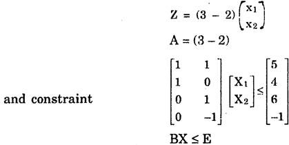
Since there are four constraints, let the variables in Dual be w1, w2, w3, w4.Then objective function of Dual becomes
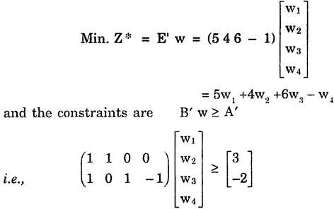
i.e w1 + w2 ≥ 3
w1 + w3 – w4 ≥ – 2 i.e. – w1 – w3 + w4 ≤ + 2
w1, w2, w3, w4 ≥ 0.
Advantages of Solving Dual Problems:
(i) Computation in simplex procedure for Dual will be easy and simple if in Primal the number of variables are lesser in comparison to the number of constraints.
(ii) Through dual one can check the accuracy of the primal solution.
(iii) It provides more exhaustive and detailed analysis for valid and economic interpretations of the solution e.g. dual values can identify critical places where expansion might be very profitable.