
Read this essay to learn about the top three methods of programming used in an organisation. The methods are:- 1. Integer Programming 2. Non-Linear Programming 3. Dynamic Programming.
Essay # 1. Integer Programming:
The optimal solution given by Linear Programming methods many times provides fractional values for the variables whereas in reality the nature of the problem may demand these values to be integers e.g. number of cars manufactured in a plant, allocation of men to different machines, number of trucks required for transportation etc.
The rounding-off the fraction values of the optimal solution from linear programming cannot guarantee that the deviation from actual values will not be large enough to retain the feasibility of the solution.
Thus we should try to evolve some method by which an integer solution is obtained without any unreasonable or arbitrary approximations. The method is known as Integer Programming. If all the variables should have integer values then it is known as Pure I.P.P. and some variables can have integer values and some can have fractional values in the solution, then it is known as Mixed I.P.P.
ADVERTISEMENTS:
If X1 , X2, X3 are the variables in the problem with
Z = C1 X1 + C2 X2 + … + Cm Xm
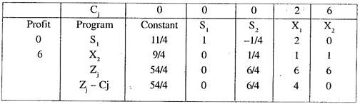
subject to the restrictions
Xj ≥ 0 for all j and can take only integer values.
ADVERTISEMENTS:
The problem is also known as Discrete Programming.
Difference between IPP and LPP:
Following are the differences between IPP and LPP:

Solution of IPP:
There are many methods to solve Integer Programming problems.
ADVERTISEMENTS:
Two most popular methods, namely:
(i) Gomory’s constraint or cutting plane method and
(ii) Branch and bound method are discussed in this section.
ADVERTISEMENTS:
(i) Gomory’s Constraint Method:
A systematic procedure to solve IPP was first suggested by Gomory in 1958. The optimum solution by this method is obtained in finite number of steps.
The method involves construction of secondary constraints after getting the optimal solution from any of the usual linear programming methods. If all the variables in the solution obtained by LPP are integers then it is taken as the solution of corresponding IPP otherwise’ some constraints are introduced eliminating some non-integer solutions, and again linear programming methods are used to find the integer optimum solution.
The constraints introduced at the later stage are known as secondary constraints. The construction of Gomory’s secondary constraints at various iterations of IPP is very important and peculiar. It needs special attention.
ADVERTISEMENTS:
The method is explained by the following example:
Example 1:
Find the optimum integer solution of the IPP
Max Z = x1 + 2X2
ADVERTISEMENTS:
s.t. 2x2 ≤ 7
x1 + x2 ≤ 7
2x1 ≤ 11
x1, x2 ≥ 0 and are integers.
ADVERTISEMENTS:
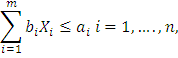
First the problem is considered as an ordinary l.p.p. and the simplex tableau at the second iteration is:

ere all Zj – Cj are positive. Hence the solution is optimal i.e. X1 = 3.5, X2 = 3.5 which are not integers.
Here the fractional part in the constant column of the simplex tableau is (1/2, 0, 1/2). We select any of X1 or X2 at this stage for constructing Gomory’s constraint. Let us consider X2 = 3.5.
Note:
If X1 and X2 were having different fractional parts, then we should have constructed the Gomory’s constraint with the variable having larger fractional part.
ADVERTISEMENTS:
Now the equation for X2 from tableau I can be written as:
(1/2) S3 + X2 = 3(1/2) = 3 + 1/2
i.e. S3 ≥ 1 is the Gomory’s constraint at this stage.
Introducing surplus and artificial variables in the Gomory’s constraint. We get
S3 – S4 + A1 = 1
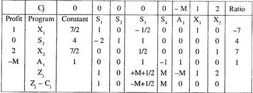
This constraint equation is introduced in the simplex tableau to get the modified simplex tableau II.
ADVERTISEMENTS:
Here S3 is the key column. Evidently S2 is entering variable and A3 is departing variable. The next Tableau III is now prepared in usual manner.
Thus all Zj – Cj, are positive. Hence the optimal solution is
X1 = 4, X2 = 3 with Max. Z = 10.
Example 2:
ADVERTISEMENTS:
Max. Z = 2X1 + 6X2
s.t. 3X1 + X2 ≤ 5
4X1 + 4X2 ≤ 9
X1 X2 ≥ 0 and are integers.
Solution:
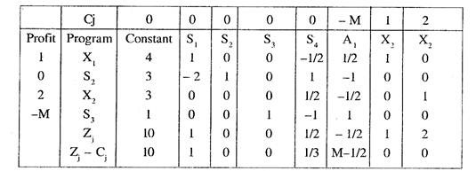
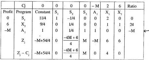
Introducing slack variables in the constraints and the, objective function and solving it by simplex method, the final Tableau giving the optimum solution is given below and the optimum solution is X1 = 0, X2 = 9/4, S1 = 11/4.
ADVERTISEMENTS:
Now S1 = 2 + 3/4
X2 = 2 + 1/4
Thus the variable S1 has the larger fractional part. So the secondary constraint is constructed with the help of row for S1 in the Tableau II i.e. we have
S1 – (1/4) S2 + 2X1 = 11/4
or (1 + 0) S1 + (-1 + 3/4) S2 + (2, 0) X1 = 2 + 3/4
ADVERTISEMENTS:
Thus examining the integral and fractional parts of the two sides, we get the secondary constraint as (3/4) S2 ≥ 3/4, i.e. S2 ≥ 1. Adding surplus and artificial variables, the secondary constraint is written as S2 – S3 + A1= 1 (Gomory’s equation).
At this stage Tableau II is now modified to get Tableau III i.e.
Here we should give priority to the artificial variable to be removed from the basis.

All Zj – Cj in Tableau IV are positive. Hence the solution is optimal. Thus the required solution is X1 = 0 and X2 = 2.
The various steps of Gomory’s method for Examples 1 and 2 can be generalized as:
(i) Formulate the given problem in a linear programming problem and find the optimum solution by any of the methods.
(ii) If the values of all the variables in step (i) are integers, then these can be taken as the solution of corresponding I.P.P., otherwise go to step (iii).
(iii) Locate the variables in the solution of step (i) with largest fractional part and using the last simplex tableau of ordinary I.p.p. write the equation for this variable.
(iv) Find the secondary constraint by comparing the integer and fraction parts of the coefficients for each variable appearing in the equation obtained in step (iii).
(v) Using surplus and artificial variables change the secondary constraint into an equation.
(vi) The final tableau of the ordinary I.p.p. is now modified by adding the new surplus and artificial variables of secondary constraint equation and its coefficient in additional row.
(vii) Find the optimal solution of the modified L.P.P. by simplex method,
(viii) If all the values in the modified solution are integers then stop at this stage, otherwise go to step (iii).
(ii) Branch and Bound Method:
It is an iterative method to find solution of IPP and can be conveniently used when the number of variables in the model are not too many. Graphical method can be used in the case of two variables. Here the solution of the problem obtained by L.P.P. can be divided or branched into a number of sub-problems and each one is solved to find the optimum solution.
The exploration of optimum in sub-regions of the original problem is known as branching. Attention is confined only to the feasible region of the original solution. Branching process terminates as soon some optimal solution is available.
The steps in the method are:
(i) Find an optimum solution, treating the problem as ordinary I.p.p.
(ii) If the solution values are integers, then the solution of step (i) is also the solution of IPP otherwise go to step (iii).
(iii) Select the variable whose value in step (i) is non-integer. There can be more than one variable in the initial solution having fractional values.
In that case selection of the variable for further branching can be done on the basis of following considerations:
(a) Select the variable with the largest fractional value.
(b) Priority can be given to a variable which represents some important decision in the model.
(c) The co-efficient of the variable in the objective function is more in comparison to other variables.
(iv) The variable selected in step (iii) is used to branch the problem into sub-problems.
(v) The branching process is continued, till optimal solution of all sub- IPP is obtained.
Example 3 is used to illustrate the procedure:
Example 3:
Solve the following I.P.P.
Max. Z = 7X + 9Y
s.t. – X + 3Y ≤ 6
7X + Y ≤ 35
0 ≤ X,Y ≤ 7
X, Y are integers.
Solution:
The problem is first solved by graphical method and the solution is
X = 9/2 and Y = 7/2
Evidently the values of X and Yare not integers. Both the variables have equal fractional part, so we select Y with largest coefficient in objective function.
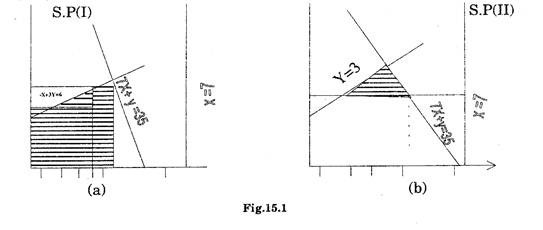
The two sub-problems at this stage can be:
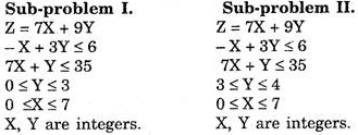
The optimum solution in both these cases (See figure 15.1) comes out to be
Y = 3 and X = 4.5
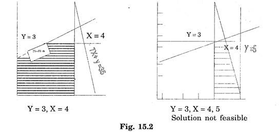
Again X is not an integer in the solution. So further branching is done taking (See figure 15.2)
0 ≤ X ≤ 4
4 ≤ X ≤ 5
Thus Y = 3 and X = 4 is the optimum solution with Z = 55
Application of I.P.P:
Some of the solutions where IPP can be effectively used are:
(i) A capital budgeting problem where the organisation wants to plan a number of products during some periods. There is limited capital available in each period and each project requires some definite investment in each period.
(ii) Ware house location problems where the firm desires to select some sites which minimises the total transportation costs.
(iii) Job-sequencing problems for determining the sequence in which the various products are to be processed on machines so as to finish the work in the least possible time.
Essay # 2. Non-Linear Programming:
Non-Linear Programming is also a technique to find some optimum solution to business problem where the restriction of linearity w.r.t. objective function as well as the constraints is not possible e.g. in actual practice a linear relationship between factors affecting profit/cost may not exist when production levels vary.
“A company faces a price-output relationship such that the lower the price greater is the sale even when price of competitive products also decreases. Also the sales volume varies disproportionately with price. Evidently the objective function in this case will be non-linear.”
Similarly many problems of Operations Research, viz. inventory models etc. may have non-linear relationships among the decision variables.
A programming is non-linear when:
(i) Objective function is non-linear but constraints are linear.
(ii) Objective function is linear but one or more constraints are non- linear. Mathematically NLP problem for m decision variables X1, X2… Xm can be defined as
Optimise F (X1, X2, …. Xm)
s.t. fi (X1, X2, …. Xm) ≤ ki, i = 1, 2, ….,
X ≥ 0, for all j
Here functions F and f can be non-linear in X’s. One of the notable characteristics of NLP problems is that the feasible region can have disjoint parts.
Methods to Solve NLPP:
There are three methods to solve non-linear programming problems namely:
I. Graphic method.
II. Gradient steepest accent method.
III. Barrier method.
In NLPP the computational procedures may not always yield an optimal solution in finite number of steps.
I. Graphic Method:
The method id illustrated by the following examples:
Example 4:
Min Z = [(X1 – 8)2 + (X2 – 4)2]
s.t. X1 + X2 ≤ 8
– 3X1 + 2X2 ≤ 6
X1, X2 ≥ 0
Solution:
The graphical solution of the problem can be obtained by plotting the objective function and the constraints (see fig. 15.3)
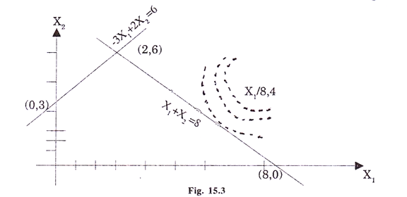
In this problem we want to find to find a point in the feasible reign which lies at the shortest distance from the centre (8, 4). Evidently the point will lie at a place where the circle is tangent to the boundary of the feasible region, in the graph, it is the point (6, 2). Thus the optimal solution is x1= 6 and x2 = 2 with Z = 2.828.
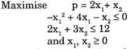
Example 5:
Solution:
Now – x12 + 4x1 – x2 ≤ 0 can be written as x2 ≥ – x12 + 4x1
Putting x2 = x12 + 4x1, we can plot the function by taking at least three points i.e.
![]()
Similarly the line 2x1 + 3x2 = 12 can be plotted by the point
![]()
The linear objective function can be plotted by taking some arbitrary value of p say 1.
![]()
The graphical representation of the problem is shown in Fig 15.4:
It is evident that the constraints points should lie on or above the parabola. F1 and F2 are the feasible regions. Point P yield the maximum value of p and lies in the region F1.
The values of x1 and x2 corresponding to the point P will give the optimum values of X1 and x2.
Note:
It can be observed that in NLP the optimum solution cannot be explored only at the corners of the feasible region.
II. Gradient or Steepest Accent Method:
(i) Non-Linear Objective Function and Linear Constraints:
Approximation techniques can be used to solve such problems. These techniques are used along with the simplex method of I.p.p. The nonlinear function is replaced by some polynomial to apply simplex method.
(ii) Non-Linear Objective Function and Non-Linear Constraints:
Here the optimum point is located at a point where the slope of the constraint should be equal to the slope of the contribution curve.
Example 6:
Optimise Z = (7.34X – 0.02X2) + 8Y
s.t. 2X2 + 3y2 ≤ 12500
Solution:
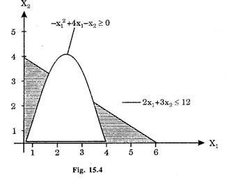
Differentiating objective function w.r.t. X we get
is the slope of the objective function.
Similarly the slope of the constraint is given by
4X + 6Y – dY/dX = 0
i.e. dY/dX = – 4X/6Y
Is the slope of the constraint.
Equating the two slopes, we get
![]()
Also from the constraint equation:

Putting this value of Y from (2) in (1), we can find the solution, giving X = 50, Y = 50 and Z = 717.
III. Barrier Method:
In this method some sort of barrier function is created. This barrier function restricts the search of optimal points inside the feasible points and make non-feasible points un-accessible. The basic condition for the application of this method is that the feasible region should be closed and bounded, which can only be possible when constraints are in the form of inequalities.
Essay # 3. Dynamic Programming:
There may be situations where a sequence of interrelated decisions may be required for the solution of the problem. Many everyday life problems needs decision making at various stages viz. inventory, allocation, and replacement problems. The technique of dynamic programming provides solution to such problems.
It is a sequential procedure where at each stage only one variable is optimized. The problem is divided into a number of sub-problems and the solutions of sub-problems are then combined to get the overall solution i.e. Optimal solution at any sequential stage = Optimal decision at the immediate stage + Optimal combination of solutions at all future stages.
The method is based on the principle of optimality which states that, “an optimal policy has the property that whatever the initial state and initial decision are, the remaining decisions must constitute an optimal policy with regard to the state resulting from the first decision.”
The solution of the problem is obtained sequentially starting from the initial stage to the next, till final stage is reached.
The following are the basic differences in DPP and LPP:
(i) DPP can be solved by sequential procedure only where-as LPP is an iterative procedure considering all variables simultaneously.
(ii) There is no standard algorithm for solving DPP where as for LPP the algorithm is well defined and always leads to an optimal solution.
Since there is no clear-cut procedure for solving dynamic programming problems, each problem requires special consideration and modification in the procedure.