
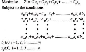
Various techniques used in Operations Research to solve optimisation problems are as follows: 1. Linear Programming 2. Waiting Line or Queuing Theory 3. Goal Programming 4. Sensitivity Analysis 5. Dynamic Programming 6. Nonlinear Programming.
Technique # 1. Linear Programming:
Linear programming is one of the classical Operations Research techniques. It had its early use for military applications but presently it is employed widely for business problems. It finds applications as resource allocation like crude oil distribution to refineries, production distribution; in agricultural works like blending fertilizers, selecting the right crop to be planted; in army such as bombers placements, troops deployment; and in finance, personnel and advertising.
Linear programming is powerful mathematical technique for finding the best use of the limited resources of a concern. It may be defined as a technique which allocates scarce available resources under conditions of certainty in an optimum manner, (i.e., maximum-minimum) to achieve the company objectives which may be, maximum overall profit, or minimum overall cost.
Linear programming can be applied effectively only if:
ADVERTISEMENTS:
(a) The objectives can be stated mathematically.
(b) Resources can be measured as quantities (number, weight etc.).
(c) There are too many alternate solutions to be evaluated conveniently.
(d) The variables of the problem bear a linear (straight line) relationship, i.e., a change in one variable produces proportionate changes in other variables. In other words, doubling the units of resources will double the profit. Problem solving is based upon the system of linear equations.
ADVERTISEMENTS:
The linear programming model may look as under:
The methods, which are commonly used to solve linear programming problems are discussed below:
(a) Graphical Method:
Simple two dimensional linear programming problems can be easily and rapidly solved by this technique. The technique can be easily mastered and shows a visual illustration of the relationships. But, as the number of products and constraints increase, it is very difficult to show and interpret the relationship (among the variables of the problem) on a simple two dimensional graph. This method can easily be applied up to three variables.
ADVERTISEMENTS:
Example 11.1. will explain how to solve a linear programming problem by graphical method.
Example 1:
A furniture manufacturer makes two products X1 and X2 namely Chairs and Tables. Each chair contributes a profit of Rs. 20 and each table that of Rs. 40. Chairs and Tables, from raw material to finished product, are processed in three sections S1, S2, S3. In section S1, each chair (X1,) requires one hour and each table (X2) requires 4 hours of processing.
In section S2 each chair requires 3 hours and each table one hour and in section S3 the times are 1 and 1 hour respectively. The manufacturer wants to optimize his profits if sections S1, S2 and S3 can be availed for not more than 24, 21 and 8 hours respectively.
ADVERTISEMENTS:
Solution:
The First Step is to formulate the linear programming model, i.e., a mathematical model from the data given above.
The model is as under:
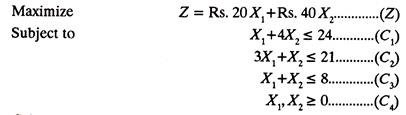
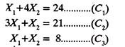
C1 is constraint No. 1 and so on.
ADVERTISEMENTS:
The Second Step is to convert the constraint inequalities temporarily, into equations, i.e.,
In Third Step axis are marked on the graph paper and are labeled with variables X1 and X2.
ADVERTISEMENTS:
Fourth Step is to draw straight lines on the graph paper using the constraint equations, and to mark the feasible solution on the graph paper. For example, taking first constraint equation.
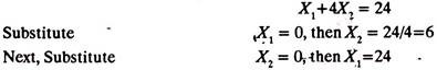
Mark the point of 24 at X1 axis and point of 6 on X2 axis. Join them. This straight line represents C1 equation. Similarly constraint equations C2 and C3 can be plotted (Fig. 11.2).

According to constraint C4, X1 and X2 are greater than (or equal to) zero, hence the marked area (region) between X1 = X2 = 0 and C1, C2, C3, represents the feasible solution.
ADVERTISEMENTS:
As the Fifth Step, a (dotted) straight line representing the equation (Z) is drawn, assuming any suitable value of Z say 120.
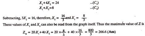
In the Sixth step, a straight line Zm is drawn parallel to the line Z, at the farthest point of the region of feasible solution, i.e., point B, at the intersection of C1 and C3. The co-ordinates of point B can be found by solving equations C1 and C3.
(b) Transportation Problem:
Transportation or Distribution methods of solving Linear programming problems aim at minimizing costs of (material handling) sending goods from dispatch stations to receiving ends. Generally, specific quantities of goods are shipped from several dispatch stations to a number of receiving centres.
Linear programming approach in such situations tends to find, how many goods may be transported from which despatch station to which receiving end in order to make the shipment most economical (least costly). Transportation technique in such problems gives a feasible solution which is improved in a number of subsequent steps till the optimum (best) feasible solution is arrived at.
ADVERTISEMENTS:
Two methods for solving transportation problems have been explained below:
(a) Vogel’s approximate method, and
(b) North-West corner method.
Vogel’s method was developed by W. R. Vogel, and gives good approximation to the solution. It provides optimum solution in simple problems. In complex transportation problems also, the first solution is obtained using Vogel’s method which is further worked upon and tested for optimality by stepping stone method or modified distribution method.
(i) Vogel’s Approximate Method:
Procedural steps:
ADVERTISEMENTS:
(a) Form the matrix based on the given problem.
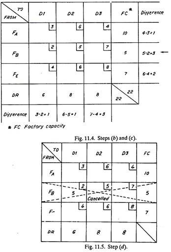
(b) Find the difference between the minimum and next to minimum cost of every column and row.
(c) Select a row or column containing the largest difference and mark it by an arrow. If the same largest value of difference in cost exists both in a column and a row, any one of two, either column or row can be selected.
(d) Mark the maximum quantity of goods in that square, of the column or row, which carries the lowest cost. This either meets all the requirements of the receiving end (DR) or exhausts the capacity of a dispatching station (FC), and thus that particular row or column is cancelled.
(e) Steps (a) to (d) are repeated until all the goods have been distributed.
(f) Stepping stone method can be used at this stage for checking optimality.
ADVERTISEMENTS:
Example 2:
An industrialist has three factories one each at Bangalore (A), Bhopal (B) and Kanpur (C) and three dealers to sell his goods at Delhi (1), Bombay (2) and Madras (3).
The cost of transporting an item from a factory to a dealer along with the number of goods (or items) available at factories A, B, E and those required by dealers 1, 2 and 3 are shown in the matrix given below:
Find the least cost of transportation.
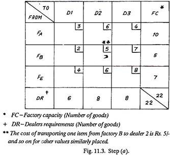
Solution: First Trial
Second Trial:
Third Trial:
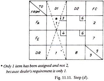
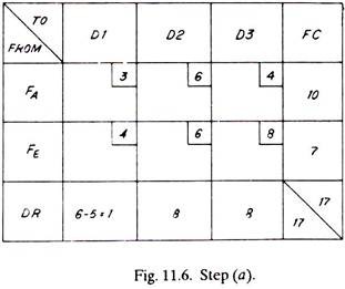
The matrix reduces to that of Fig. 11.12 as given below:

The only alternative now left is to transport to dealer No.2, one item from factory A and seven items from factory E (shown dotted)

It may or may not be optimum feasible solution. This has to be checked by stepping stone method for optimality.
When all the goods as distributed from factories to dealers are shown in the original matrix of Fig. 11.3 it takes the shape of Fig. 11.13. It is evident that from factory, 4, one item each is sent to dealer No. 1 and dealer No. 2 and eight goods are shipped to dealer No. 3 and similarly from factories B and E. The optimum minimum cost of transportation or distribution of goods is equal to
(1×3) + (1×6) + (8×4) + (5×2) + (7×6) = Rs. 93.
As done above, it is not necessary to construct separate matrix for each step when solving such a problem. Once the practice is attained, many steps may be combined together to arrive at the final results in a much shorter duration.
(ii) North-West Corner Method:
Figure 11.14 shows the matrix of Fig. 11.3 taken from the Vogel’s method.

The North-West Corner method derives its name from the fact that initial allocation of resources is started from the north-west corner of the matrix. Ignoring other things (i.e., cost) and simply considering the factory capacity and dealer’s requirements, the minimum (number of goods) of the two (i.e., FC & DR) is placed in north-west corner; for example, though factory, A can supply 10 items, dealer 1 needs only 6.
Therefore, 6 items are marked in the north-west corner, (Fig. 11.15). Next it is just ‘stair stepping down’ the matrix from north-west corner to south-east corner and allocating the goods. For example, by placing 6 goods in the AW corner, the requirements of dealer 1 are over, but dealer 2 needs 8 goods. To him, 4 can be supplied from factory A and naturally 4 from factory B if one has to step down the stairs in the matrix. In this manner the initial north-west solution is marked in the matrix, Fig. 11.15.

This initial solution can be improved by using Stepping Stone Method developed by Cooper and Charnes. The empty or open squares are called Water Squares and the squares having assignment of goods are known as Stone Squares.
The stepping stone method is explained below:
The criteria of judging whether the solution has been improved or not is based upon the fact whether the transportation cost has been reduced or not. The cost of transportation for the initial solution by north-west corner allocation is
(6×3) + (4×6) + (4×5) + (1×7) + (7×8) = Rs. 125.
The stepping stone procedure involves stepping or shifting some goods to an empty square from a stone square if it can bring about a saving in transportation cost. The number of goods to be shifted is restricted by the number of goods available (FC) and goods required (DR). For doing so, first of all a closed loop, (of 4 or more squares is imagined) having one empty square and rest all stone squares, is selected, as in Fig. 11.15.
Only one item can be moved from square A to squared, only 3 will be accommodated in square C, and it will become 5 in square D. When one item leaves squared it means the transportation cost is reduced by Rs.7 so it is marked +ve. Since one item goes to square B, the transportation cost increases by Rs.4 and it is marked + ve.
And naturally for balancing FC and DR one item leaves square C and one item goes to square D and they are marked -ve and +ve respectively. Next, it is estimated whether by this shifting has there been any saving in the transportation cost or not. This is Rs. -7 + 4 – 6 + 5 = – 4, which (being negative) shows that transportation cost has decreased by Rs. 4 per item. Fig. 11.16 shows, thus modified matrix. The total cost of transportation is
(6×3) + (3×6) + (1×4) + (5×5) + (7×8) = Rs. 121.
The total cost of transportation is Rs. 121 against Rs. 125 (Fig. 11.15) which shows an improvement.
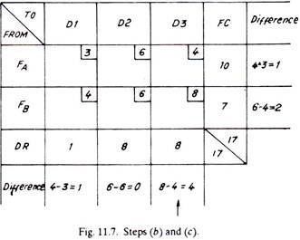
Again, another loop is tried which shows a saving in the transportation cost. This loop is marked in Fig. 11.16. The saving in this case will be (+ 6 – 8 + 4 – 6 = – 4) of Rs. 4 per item. In this loop 3 goods can be shifted from square C to square £ and corresponding adjustments in the goods of squares F and B will be done in accordance with the restrictions imposed by factory capacity (FC) and dealer’s requirements (DR). The second improved solution is given in Fig. 11.17. The total cost of transportation is Rs.109 which when compared with earlier values shows improvement.


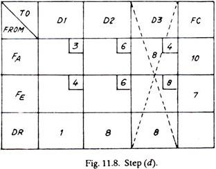
Another loop which promises saving has been marked in Fig. 11.17. The saving in this case will be of (+ 4 – 8 + 4 – 3 = – 3) Rs. 3 per item. Four items can be shifted from square F to square H and accordingly the number of items can be adjusted in squares B and G. The third improved matrix is shown in Fig. 11.18. The total cost of transportation being Rs. 97 which shows an improvement over the previous solutions.

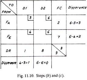
Saving can further be achieved by considering the loop marked in Fig. 11.18. The saving in this case is of Rs. (+ 2 – 4 + 6 – 5 = -1) one per item and 4 items can be shifted from square H to square I, etc. This improved matrix is shown in Fig. 11.19 and the total cost of transportation is Rs. 93 which is a further improvement.

Still, a number of more loops as shown in Fig. 11.19 can be tried but it is found that they do not do any saving rather they increase the total cost of transportation. Hence we take the solution of Fig. 11.19 as Optimum Feasible Solution.
The same problem was solved earlier by Vogel’s Method and the solution found was marked in Fig. 11.13. Though the two solutions (Fig. 11.13 and 11.19) differ as regards the distribution of goods from factories to dealers, yet the total cost of transportation (Rs. 93) remains the same. Hence both the methods, i.e. Vogel’s method, and Stepping Stone method have optimised the transportation or distribution cost.
Transportation Problems (Cost Matrix) With Unequal Supply And Demand:
Problem solved under Example 11.2 had total factories capacity of 22 goods and the dealer’s requirements were also 22; but it rarely happens in real situations.
It is quite liable that the supply and demand may not be equal. Such problems are dealt in the following way:
Assume the matrices as under [Fig. 11.20 (a) and (b)].


Such problems are solved exactly in the same manner as described previously, except that the original matrices of Fig. 11.20 (a) and (b) are adjusted to the matrices of Fig. 11.21 (a) and (b) respectively before using Vogel’s method or North-West Corner method. The adjustment is carried out by using Dummy factories or Dummy dealers to equalise (FC and DR) supply and demand. These dummy entities are assigned zero transportation cost as the goods will never be distributed.
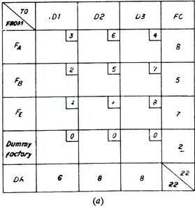
In Fig. 11.21 (a), a dummy factory with an output of 2 goods has been added which equalises total factory capacity and total dealer’s requirements. Similarly in Fig. 11.21 (b) a dummy dealer has been added and with his requirements of 2 goods, the total supply and demand becomes equal. Now the matrices can be solved by Vogel’s method or North-West Corner method.

Profit Matrix with Equal Supply and Demand:
Example 11.2 used a Cost Matrix as it contained values of transportation costs of goods and the purpose was to minimize total transportation cost. If transportation cost values are replaced by Profit values (Rs.), then the total profit which a firm will get by transporting different number of goods to different places can be Maximised.
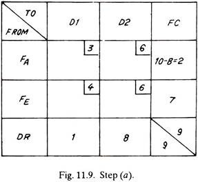
Fig. 11.22 shows a profit matrix, according to which factory A earns a profit of Rs.4 for each item which is sent to dealer 1. But it earns Rs. 8 and Rs. 6 respectively if the same item is sent to dealers 2 and 3. Similarly factories B and E earn different amounts of profits by sending items to three different dealers. The problem before the factories owner is-how many goods from which factory should be sent to which dealer so that he earns the maximum profit?

The first step in solving such a problem is to convert the Profit Matrix into a Cost Matrix as in Fig. 11.21. The maximum profit (Fig. 11.22) is Rs.8 which is assumed equal to Zero Cost and costs for all other squares are calculated by subtracting their profits from Rs.8. For example, for square A, B and C the profits are Rs.4, 5 and 1, and therefore the cost will be Rs. (8 – 4) = 4, (8 – 5) = 3 and (8 – 1) = 7 respectively.
The cost can now be minimized by the methods explained earlier. After optimum assignments have been made in different squares, the cost figures in different squares are replaced by profit figures as those of original profit matrix, Fig. 11.22. Number of goods in each stone square is multiplied by the profit figure of that square. When all such multiplied profit values are added, it gives the optimum profit.
Profit Matrix with Unequal Supply and Demand:
Fig. 11.22 of profit matrix has supply of goods equal to their demand, i.e., 20 and 20. If due to some reasons FC becomes 18, but DR remains 20 or DR changes to 17 and FC remains 20 then what should be done.
The procedure is simple and is given below:

Step-1:
Draw the profit matrix.
Step-2:
Equalise supply and demand by inserting a dummy factory or a dummy dealer with zero profit value in each square.
Step-3:
Change over to cost matrix.
Step-4:
Minimize the cost by the methods explained earlier.
Step-5:
After getting optimum assigned values (of goods) convert cost matrix into profit matrix.
Step-6:
Calculate the optimum profit.
Degeneracy:
A Transportation problem can only be optimized if it contains (m + n -1) stone squares (i.e., squares having assignment of goods), where m is the number of rows and n is the number of columns in the matrix (refer Fig. 11.28).

If the number of stones is less than (m+n-1) values, then the closed path to evaluate the water squares cannot be traced and the matrix is said to be degenerate. The first step, therefore, in optimising any matrix is to count the number of stones and to continue the solution in a degenerate matrix, it is necessary to increase the number of stones to (m + n- 1). This is done by adding a dummy stone, ϵ, in a water square. The dummy stone is merely a device to permit the solution to continue. It is inserted in the greatest profit (or least cost) square on the path that created the degeneracy.
The infinitesimal quantity, ϵ, which is assigned to a promising unoccupied cell has the unusual but convenient properties of:
(1) Being large enough to treat the cell in which it is placed as occupied, and
(2) Being small enough to assume that its placement does not change rim conditions. Supply and demand (quantities) entries are called rim conditions. They correspond to the constraints provided.
Degeneracy can develop in either an initial solution itself or in a revised solution during the process of optimization. In both cases the treatment is the same. One or more cells receive epsilon (ϵ) allocations to make the total number of occupied cells equal to (m + n – 1) . The cells to receive ϵ allocations should be carefully chosen because a transfer circuit cannot have a negative epsilon stepping stone. The reason, of course, is that you cannot subtract a unit from a cell ‘that contains only an infinitesimal part of a unit. Therefore, epsilon quantities should be introduced in cells that accommodate the solution procedures.
1 + ϵ = 1
1 – ϵ =1
ϵ – ϵ = 0
The following example will explain, how to optimize a degenerate solution:
Example 3:
A company has three factories and five dealers. With the following matrix, minimize the transportation cost. The matrix shows an initial solution which is degenerate
Solution:
The initial solution is degenerate owing to 6 instead of m + n – 1 = 3 + 5 – 1 =7 occupied cells.
A logical improvement is to eliminate the high cost FA-D3 route. The unoccupied cell FB-D3 makes a good starting point. In the existing degenerate condition, it is impossible to make a stepping stone circuit around FB—D3. An epsilon (ϵ) quantity must be introduced. Epsilon could be added to FB – D1 to complete a transfer circuit as shown in Fig. 11.29, but the epsilon stepping stone is negative and consequently allows only an inconsequential transfer.

By placing epsilon in FA-D2, it becomes a positive transfer dell in the circuit + (FB-D3) – (FA– D3) + (FA-D2) – (FB-D2) or (+16-30+24-14) = -Rs. 4 cost or Rs. 4 saving results from the transfer of one unit (Fig. 11.30).

Hence the revised solution is as follows (Fig. 11.31).

In first revised solution (Fig. 11.31), m + n – 1 = 3 + 5 – 1 = 7 and the occupied cells are also 7, hence the degeneracy is eliminated.
Now, the problem can be solved as usual as explained earlier, however, degeneracy is to be checked after every revision. Trying another loop for minimization of cost (Fig. 11.31).
+ 16 – 20 + 18 – 16= — Rs. 2.
Thus, second revision is shown in Fig. 11.32.

The second revision is the final optimal solution; all remaining routes/loops exhibit greater transfer costs. Thus, the minimum transportation cost = (16×14) + (1×24) + (5×16) + (17×14) + (1×16) + (15×18) + (9×20)
= Rs. 1032; which is Rs. 27 less than the transportation cost (Rs. 1059) of the initial (degenerate) solution.
Fundamentals of Simplex Procedure:
The simplex method was first described by Dr. G. B. Dantzig in the year 1947 and later on, due to further developments in it, it has become an excellent technique for solving linear programming problems. It provides an orderly approach to the linear programming (e.g., business) problems having dozens of variables. Problems which cannot possibly be solved with graphical technique, for them the simplex method is an alternative approach. Unlike graphical method, the simplex method uses algebraic equations.
The simplex method can handle any number of activities and can solve even those equations which have more number of unknowns than the equations. Fundamentally, the simplex procedure requires to make a table. Variables and constraints are entered into it and are subjected to a regular algorithm to arrive at the optimum solution. Once the simplex table for a problem is established, the procedure leading to optimum solution is just mechanical.
The simplex method, as compared to transportation method is more general as Regards the application and is employed where transportation method cannot.
Simplex Procedure:
(a) Express the problem as an equation.
(b) Express the constraints of the problem as inequalities.
(c) Convert the inequalities to equalities by adding slack variables.
(d) Enter the inequalities in the so-called simplex table. A simplex table is given in Fig. 11.33.

(e) Complete the simplex table.
(f) Calculate contribution lost and net contribution and mark them on the simplex table.
(g) Locate highest value of net contribution and mark it by an arrow.
(h) Divide the quantity column values by the corresponding values of the column marked by arrow and obtain the respective figures (values).
(i) Select the smallest non-negative value amongst these figures to determine the row to be replaced.
(j) Compute all the values for the new row.
(k) Compute the values for the rest of the rows.
(l) Calculate contribution lost and net contribution and mark them on the simplex table.
(m) Repeat steps from (h) to (l) till there is no positive value of net contribution or net profit. This implies that nothing more can be introduced into the mix to increase the profit and hence it is the Optimum Solution.
Example 4:
A furniture manufacturer makes wooden racks (X) and cots (Y). These products are completed in two sections. Each rack contributes a profit of Re. 1 and each cot of Rs.5. In first section each rack requires 5 hours and each cot 6 hours of processing. Similarly in section number 2 each rack has 3 hours and each cot has 2 hours of work on them. The manufacturer is interested to optimise his profits if the two sections can be availed for not more than 30 and 12 hours respectively.
Solution:
The Problem can be expressed as follows:
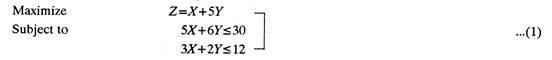
The inequalities can be removed by adding slack variables. Slack variables represent unused time in each section which yields no profit, i. e., which contributes nothing towards profit. Since same variables should appear in all the equations, those variables having no effect on an equation are given a zero coefficient, for example, (1) above is are rewritten as, Maximize Subject to
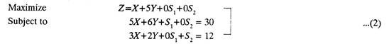
From the data given in (2), the simplex table (Fig. 11.34) is constructed.

In the initial solution (Fig. 11.34) there is no output, all the time is unused and there is no contribution or profit, i.e., initial solution is zero profit (PTM) solution. Till this point, steps up to (f) have been completed.
Step-g:
The highest-value of net contribution is 5 and has been marked by an arrow (Fig. 11.34).
Step-h:
30/6=5
12/2=6
Step-i:
Value 5 is selected.
Step-j & k:
Selecting value 5 means -Y and its profit will replace S1, and its zero profit. Divide row (D) by 6 throughout and rewrite.

Step-m:
On checking the equation (j), it is found that there is no positive value of net contribution (NC). Hence it is the Optimum Solution. The optimum profit Z = Rs. 25, (the PTM value marked).
It was a simple problem which could be optimized in the second solution. More complex problems involve a number of iterations.
Technique # 2. Waiting Line or Queuing Theory:
The credit of original work on Queuing theory goes to A. K. Erlang. He started, in the year 1905, to explore the effect of fluctuating service demand on the utilization of automatic dial equipment. But today, a wide variety of problem situations can be described by waiting line model.
A queue or a waiting line is something very common in everyday routine. There is a queue for bus, queue at ration shop, queue for cinema ticket and where not. Standing in queue wastes a lot of otherwise useful time. Besides everyday experience, queues can be seen on the shop floor, where in-process goods wait for next operation or inspection or wait for getting moved to another place. Such delays in the production lines naturally, increase production cycle duration, add to the product cost, may upset the whole system and it may not be possible to meet the specified delivery dates thereby annoying the potent customers.
A queue is formed whenever the number of arriving items is more than the number which can be processed. For example, if one hundred hand tools reach electroplating section per unit time and only eighty can be plated within that duration, naturally a queue will be set up in which a number of hand tools will be waiting for getting plated.
Waiting lines if (economically) cannot be completely eliminated, they can atleast be reduced by optimizing the number of service stations, or by adjusting the service times in one or more service stations.
Waiting line theory or queuing theory is used to solve Queue Forming situations, for example, in post offices, banks, hospitals, telephone booths or exchanges, etc. Queuing Theory analyses the feasibility of adding facilities (equipment, manpower) and assesses the amount and cost of waiting times. In general, this theory can be applied wherever congestion occurs and a waiting line or a queue is formed.
The purpose in such situations is to determine the optimum amount of facilities (manpower, machinery, etc.) Queuing theory helps finding lack of balance between items coming and going. It gives information about peak loads. It mathematically relates the length of queue and waiting time and the controllable factors, such as number of service stations or the time taken to process each article. It can also tell, how often and how long the items or persons in queue will probably have to wait.
Queuing theory mathematically predicts the way in which the waiting line will develop over given periods and in turn helps allocating facilities to deal the situation efficiently.
In order to build a mathematical model for a queue forming situation, i.e., where items or persons arrive in a random manner, are processed or treated (processing time is again a random variable) and then leave, following information is required:
(a) Distribution of gaps between the arrival of items. Say a telephone call comes after every ten minutes.
(b) Distribution of service times. Say every time a telephone talk continues for three minutes.
(c) The priority system.
(d) The processing facilities (It may be a doctor or a mechanic).
Most waiting line models assume a specific distribution of arrivals (say poisons distribution) and service times (say exponential). Knowing the above-mentioned four points (model) the waiting situation can be studied and analyzed mathematically.
Structures of Queue Forming Situations:
(1) Arriving units or persons form one line and are serviced through only one facility. For example, persons are standing in queue at the post office window to collect stamps, etc., and there is only one clerk sitting at the window for selling stamps. This is called single channel, single phase case, Fig. 11.36 (1).
(2) Arriving units or persons form one line but there are more than one service facility or service stations, as in a barber shop with more than one barber working at a time. This is a multichannel, single phase case, Fig. 11.36 (2).
(3) In another structure called single channel multiple phase case, arriving units again form one line but there are a number of service stations in series, Fig. 11.36 (3).
(4) Lastly, in multichannel multiple phase case there are two or more parallel servicing lines, Fig. 11.36 (4). Example-checkout counters of a super-market.

Assumptions Involved in Waiting Line Theory:
As regards the treatment of queuing theory in this chapter, the following assumptions are made:
(a) There is only one type of queue discipline-that is first come, first served. A unit in queue will immediately go to the service station as soon as the station is free.
(b) There are steady state (stable) conditions, i.e., the probability that n items are in queue at any time, remains the same with the passage of time. In other words at all times the number of items in the queue remain same; the queue does not lengthen indefinitely with time.
(c) Both, the number of items in queue at any instant and the waiting time experienced by a particular item are random variables. They are not functionally dependent on time. The problem thus reduces to estimate the average length of the queue at any instant, etc.
(d) Arrival rates follow Poisson distribution and service times follow exponential distribution. This situation, referred as Poisson Arrivals and Exponential Service Times, holds good in number of actual operating situations.
(e) Mean service rate µ is greater than mean arrival rate M.
Poisson Arrivals and Exponential Service Times:
Poisson Arrivals:
From the studies conducted by Nelson on Arrival, service time and waiting time distribution of a job shop production process; by Eastman Kodak Company and by O. J. Feorene, etc., it can be safely concluded that in actual real situations the distribution of arrival rates do not significantly differ from the Poisson distribution. Poisson distribution assumes that an arrival is completely independent of other arrivals, i.e., they are completely random.
Unlike Normal and Exponential distribution, the Poisson distribution is a Discrete Distribution. In other words, the possible values of the random variables are separated, i.e., discrete—for example, number of good mangoes in a basket, number of heads in N tosses of a coin, etc.
Poisson distribution is shown in Fig. 11.37 and a few of its properties are given below:

Exponential Service Times:
The results of the studies conducted by Nelson and Brigham, show different results. According to Nelson, the Exponential model does not fit the actual distributions adequately. According to him, other (mathematical) distributions such as hyper-exponential and the hyper-Erlang were better descriptions of the real world distributions. But, Brigham showed that service time at a tool crib was nearly exponential distribution. One has to be very careful before assuming the type of distribution.
Though Exponential distribution does not represent large number of situations, it is used even then because of the simplicity of the mathematical treatment and derivations involved. Other distributions may make the mathematical development too complex and it may become necessary to solve the problem by simulation (Monte-Carlo) techniques.
Unlike Poisson distribution, Exponential distribution is a Continuous Distribution. The random variables involved range over continuum of values such as, temperature in the morning, the time between two events etc. k (X-axis) can take both integer, and fractional values, so that the distribution becomes continuous.
Fig. 11.38 shows Exponential distribution and a few of its properties are given below:

Equations Governing the Queue:
Let, n = number of units in the system (total number-in queue as well as under service).
Pn = Probability that there are n units in system at any time.
M = Mean arrival rate.
µ = Mean service rate.
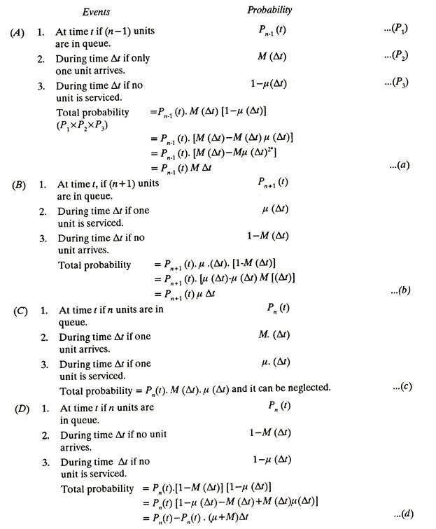
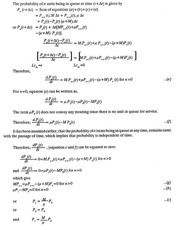
Knowing the probability of n units in the queue at any time t, the probability of getting n units in time (r + ∆t) can be calculated by summing up the probabilities of the following four mutually exclusive events (A, B, C and D).
The following examples will give an idea as how to solve waiting line problems:
Example 5:
On a telephone booth, average time between the arrival of one man and the next is 10 minutes and the arrivals are assumed to be Poisson. The mean time of using the phone is 4 minutes and is assumed exponentially distributed.
Calculate (1) the probability that a man will have to wait after he arrives; (2) the average length of waiting lines forming from time to time; (3) by how much the flow of arrivals should increase to justify the installation of a second telephone booth. Assume that second booth can be provided only when a person has to wait minimum for 4 minutes for the phone.
Solution:
In 10 minutes there is one arrival.
Therefore in 1 minute there are 1/10 arrivals.
M = 1/10 = 0.1 arrivals per minute.
Service time is 4 minutes per arrival.
Therefore µ = 1/4 or 0.25 services per minute.
(1) P, the probability that one has to wait = 1 – P0
From equation (i)
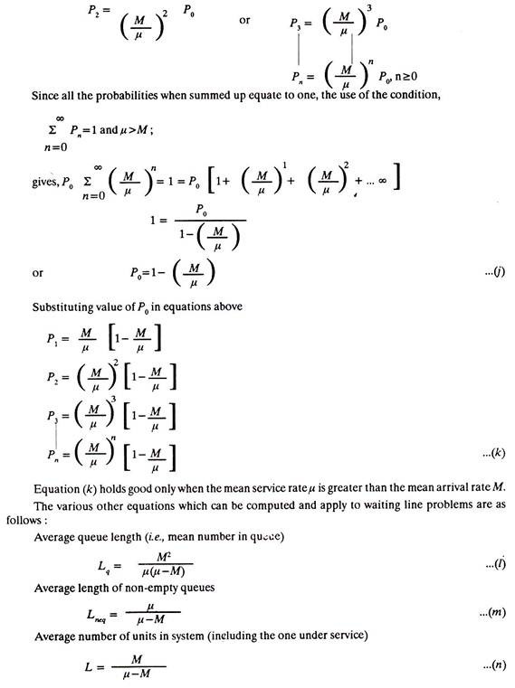
P0 = 1-M/µ or 1-P0 = M/µ
Thus P from (1) above=1 – P0 = M/µ = 0.1/0.25 = 0.4
(2) The average length of waiting lines or queues that from time to time, or average length of nonempty queues is given by equation (m)
Lneq = µ/µ-M = 0.25/0.25-0.1 = 1.66 persons
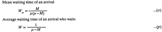
(3) Mean waiting time of an arrival is given by equation (o)
Wm = M/µ(µ-M)
4 = M/0.25(0.25-M1); M1 being the new arrivals per minute corresponding to mean waiting time of 4 minutes, which gives M1 = 0.125 arrival per minute.
Thus the flow of arrivals must be increased from 0.1 per minute to 0.125 per minute or 0.1 x 60, i.e., 6 per hour to 7.5.or say 8 per hour.
Applications of Queuing Theory:
Queuing theory is applicable wherever a queue forms.
A few places where such situation may occur are as follows:
(a) Super markets,
(b) Post offices,
(c) Telephone switch-boards,
(d) Petrol pumps,
(e) Stores/warehouses,
(f) Toll houses,
(g) Repair and Maintenance Sections,
(h) Hospitals/Doctors,
(i) Ports (Ships entering),
(j) Computer centres,
(k) Assembly lines,
(l) Bus stops,
(m) Auto traffic at road or railway crossings,
(n) Job shop production process,
(o) Insurance Companies,
(p) Banks, and
(q) Tool crib.
Queuing theory helps in deciding the number of persons, equipment or other facilities required in above situations for their efficient functioning.
Technique # 3. Goal Programming:
Goal programming is a special approach to linear programming. This approach is capable of handling a single objective with multiple sub objectives. Higher level objectives can be maximized or minimized first, before lower level objectives are brought into the final solution. Hence preference is given to those objectives that are of greater significance to an organization. These objectives are called goals.
The Methodology of Goal Programming (GP):
To solve a goal programming problem, we follow a series of iterative steps. As with the simplex method of linear programming, an algorithm is employed until the final answer is determined.
The specific steps that we must follow to solve the GP problem are:-
Step-1: Review Model formulation for appropriate deviational variables:
Since we need to rank the goals in order to formulate GP problems, we require a type of variable that can be used to reflect the underachievement or overachievement of stated goals, and variables of this type are termed deviational variables.
Although the procedures followed here for developing variables and constraint equations in goal programming problem are the same as those in the simplex method of linear programming, deviational variables must be included, where necessary, to describe the problem being formulated.
Step-2: Solve using the Simplex Method (Modified):
A GP problem can be solved using the iterative procedures of the simplex method of linear programming. If the problem features a single goal with multiple sub-goals, the tableau structure need not be changed.
On the other hand, if the problem treats multiple goals with multiple sub-goals, one additional Zj row and Cg-Zj row must be added for each priority factor (i.e., for P1, P2, P3…. ). This enlarged tableau structure permits evaluation of all goals that have bearing on the problem’s solution. Note that the answer obtained by using the simplex method provides the best solution in terms of coming as close as possible to reaching all of the intended goals.
When starting doing computations for the simplex method, in the first step, the potential loss in the objective function from one unit of each variable entering the basis is computed and written in a row called the Zj row (where j is the variable column). Second, since the gain is known for one unit of each variable in the objective function row (called the Cj row), the net result of a gain minus its loss for all the basic and non-basic variables will be values in the Cj-Zj rows.
Goal programming, like linear programming will call for sensitivity analysis to answer managerial What if questions.
Applications of Goal Programming:
(1) Selection of organization objectives:
Helps determine what type of objective(s) and strategies the manager should employ to realize the vast potential of an organization’s resources.
(2) Establishing sales goals:
Assists the manager in determining the time to be spent on established customers versus new ones.
(3) Aggregate production planning:
Aids the manager in planning and scheduling production quotas for the coming period.
(4) Aggregate planning of work force:
Assists in minimizing payroll expenditures through more effective hiring and layoff procedures, overtime practices and the like.
(5) Multiplant scheduling:
Analyzing multiplant scheduling problem
(6) Capital project evaluate:
Helps the manager determine what investment amounts to place on new capital projects.
Technique # 4. Sensitivity Analysis:
If a manager is given the ability to produce grange of possible outcomes in response to the request for an estimate this will reduce the worry in the mind of the manager who must produce the estimate. If the range reveals that most favourable estimate produces a favourable outcome, still there is no worry. But if the least favourable estimate produces an unfavourable outcome, there is indeed the great need to worry because if this least favourable, bottom side estimate should come to pass then the firm could be in trouble.
Therefore part of the process of forecasting must be to highlight any such extremely critical or sensitive areas by seeking to answer a series of what if… ? questions e.g. what would happen to profitability and to liquidity if sales fell by 25% ? What if customers took three months to pay their accounts instead of one month? And so on. This aspect of forecasting is called sensitivity Analysis.
The object of sensitivity analysis, by iterative combination of all possible outcomes within the range of estimates submitted, is to isolate within the forecast those critical factors or key variables, variations in which are likely to have the most critical impact upon the financial fortunes of the firm. Management attention must then be focused on these key variables because these are the killer areas: areas where it is worth seeking more information in order to improve the quality of the best guess estimate; areas where some form of insurance might be sought; areas where subsequent vigilance in the monitoring both of forecasting assumptions and of actual cash flows must be strongest in order to give the earliest warning of an impending financial crisis.
It must be stressed that sensitivity analysis is a relatively simple and unsophisticated concept: all it implies is that several forecasts are produced from a range of estimates fed into the process instead of producing one forecast from single point estimates. The firm is thereby more easily able to ascertain under what combination of circumstances it might be exposed to risks which it would prefer not to face. At the best these risks might represent a break in the continuity of cash flows so as to frustrate certain management decisions considered to be essential to the firm; at worst they might represent insolvency.
Technique # 5. Dynamic Programming:
Dynamic programming is a newly developed mathematical technique which is useful in many types of decision problems. Many business problems, as a rule, share a common characteristic: they are static. That is, the problems are stated and solved in terms of some specific situation that occurs at a given moment. Other problems, however, are concerned with variations that occur over time or through some sequence of events and to solve such problems, another Management Science, called Dynamic Programming is used.
Dynamic programming is an extension of the basic Linear Programming technique. When a problem is considered with reference to its parameters varying over time, techniques like Linear Programming, are no longer applicable and the Dynamic Programming has to be used as it includes the time element. Dynamic Programming was developed by Richard Bellman and G.B. Dantzig, whose important contributions to this quantitative technique were first published in the 1950s.
In its simplest sense, dynamic programming can be thought of as an attempt to break large, complex problems into a series of smaller problems that are easier to solve separately. In other words, dynamic programming divides the problem into a number of sub-problems or decision stages. General recurrence relations between one stage and the next describe the problem. There are number of decision stages and at each stage there are several alternate courses of action. The decision generated by stage one, acts as conditions of the problem for stage two and so on.
In other words, at each of the several stages there is a choice of decisions and the decisions, initially taken affect the choice of subsequent decisions. The various rules of decision making can be established after considering the effects of each decision (separately) and the optimum policy for further decisions. The basis of dynamic programming is to select the best amongst the final possible alternative decisions. This process is then repeated, ignoring all those alternatives which do not lead to selected best (optimum).
The best sequence of decisions can thus be defined, by repeating the above procedure. Dynamic programming is also concerned with problems in which time is not a relevant variable; for example, in the case where a decision must be made as to the allocation of resources in fixed quantity among a number of alternative uses. A dynamic problem approach is advantageous for solving problems where a sequence of decisions must be made. Even though incorrect or less-than-optimal decisions may have been made in the past, dynamic programming enables one to still make decisions for future periods.
The following basic terms and concepts are central to the theory of dynamic programming:
1. State Variables:
These are variables whose values specify the conditions of the process. The values of state variables tell us all we need to know about the system for the purpose of making decisions. For example, in a production problem, we might require state variables that relate to plant capacity and present inventory. The lesser the number of state variables, the easier is to solve a problem.
2. Decision Variables:
These constitute opportunities to change the state variables (possibly in a probabilistic manner), and the net change in the state variables over some time period will be subject to considerable uncertainty. The returns generated from each decision will depend on the starting and ending states for that decision, hence they will add up as a sequence of decisions. Depending on circumstances, the task is to make decisions that will either maximize or minimize a certain objective.
3. Stages:
The ability to make decisions about some problem at various stages (or points in time), is an important feature of dynamic programming problem formulation. In problems where decisions are made through a series of events, stages are represented by the events. At each stage in a problem, a decision is made to change the state and, thereby, maximize or minimize a certain objective. Then, at the next stage, decisions are made using the values of the state variables having resulted from the preceding decision and so forth.
The solution is ultimately reached by moving backwards (or forwards, if desired), stage by stage, and determining the optimal policy (i.e., set of decisions) for each state variable at each stage in time, until the overall optimal policy has emerged in the final stage.
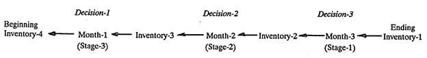
To see how the above explained concepts are applied in a problem, consider the following question:
“What is the minimium cost production schedule for the next three months” ?
If the state variable is inventory,
the decision variable is the level of production, and
each month is a stage, then
the dynamic programming formulation for this problem’s sequential, multistage decision making is as follows:
4. Objective:
As with other Management Science models, a dynamic programming problem requires an objective (i.e., an objective function). A typical objective may be to maximize total profit or to minimize total cost.
The Methodology of Dynamic Programming:
The following steps constitute the basic methodology of dynamic programming:
Step-1: Determine an appropriate mathematical modelling technique:
In this first step of the methodology of dynamic programming, the appropriate mathematical technique, either standard or custom-made, for solving the problem is selected.
Step-2: Solve for the objective function using a multistage problem solving approach:
To employ the multistage problem-solving approach, it is necessary to break the problem down into component stages. Using the appropriate mathematical technique, the solution is then obtained by moving backwards from the problem’s desired end results, stage by stage, to its beginning. In the process, an optimal set of decisions is determined at each stage which can guide the manager in decision making over time or through a series of events.
Applications of Dynamic Programming:
Dynamic programming finds application in the following areas:-
1. Scheduling production.
2. Scheduling equipment and machinery overhauls.
3. Smoothing employment (of workers) in an environment with widely fluctuating demand.
4. Determining equipment replacement policy.
5. Maximizing expected sales by determining the best combination of advertising media to use and the best efficiency of use, within a certain budget constraint, to maximize expected sales.
6. Allocating capital funds to new ventures for maximizing profits over the long term.
7. Evaluating investment opportunities: Determines the most profitable investment of resources or the best alternative among given opportunities.
8. Determining the best long-range strategy for replacement of depreciating assets.
Difference between Linear Programming and Dynamic Programming:
(1) Dynamic programming is characterized as a multi-stage decision making process that spans time intervals; however, the intervals may consist only of stages in which the problem is solved. Linear programming, conversely, gives a solution that will pertain only to one time period within given capacity, quantity and contribution (or cost) constraints.
(2) With dynamic programming, wrong decisions in the past will not prevent correct decisions from being made either at present or in the future.
In essence, dynamic programming permits one to determine optimal decisions for future time periods, regardless of any earlier decisions, unlike linear programming, which requires constant updating of any values obtained in order to reflect the current constraints necessary for an optimal answer.
(3) Dynamic programming is more powerful in the sense of a concept than linear programming, but weaker as a computational technique.
(4) Dynamic programming is similar to calculus, whereas linear programming is analogous to solving sets of simultaneous linear equations.
(5) Dynamic programming takes a quite different form than linear programming; whereas certain rules must always be followed in the iterative process of linear programming, dynamic programming uses whatever mathematics are deemed appropriate to the solution of the problem.
Technique # 6. Nonlinear Programming:
The underlying theory for much of the research done in non-linear programming was presented in a paper by Kuhn and Tucker in 1951. However, the major thrust in solving real-life nonlinear programming problems was made after 1960.
In the case where either the objective function or the constraints are non-linear, use is made of non-linear programming techniques. Non-linearities exist, for example, when a firm must lower prices to induce more people to buy. In many of these nonlinear situations, linear programmes have been used as approximations and have proved to be adequate.
However, with the increase in sophistication of the users, together with availability of non-linear computer routines, there will be a marked increase in the use of this technique. There are problems of business and industry where the assumption of linearity is not quite valid.
In transportation problems, for instance, there are bulk transportation rates which are cheaper than the regular transportation rates. These rates are applicable if the amount transported is above a certain quantity. Thus, the objective function no longer remains linear, but becomes a non-linear function of decision variables.