After reading this article you will learn about the decisions taken under certainty and uncertainty.
Decision under Certainty:
The decisions may be taken when the problems are under certainty i.e., where a complete knowledge about the nature of future conditions is known. Let us take a simple example.
It is not uncommon for constructing firms to set up service facilities in an area in which they have unusual temporary activities. Many times they come across to find the economy of setting up such facilities and the economy of various locations within the area.
Example 1:
ADVERTISEMENTS:
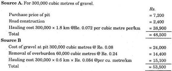
If a firm having a contract to built a dam across a river requiring 300,000 cubic metres of gravel, found two feasible sources whose characteristics are given below:
Solution:
ADVERTISEMENTS:
Now to make decision on the basis of economy, the cost of securing the required gravel from either source should be determined.
Thus the decision must be in favour of Source A on the basis of economic analysis.
Decision under Uncertainty:
Further, as everybody knows that now-a-days a business manager is unable to have a complete idea about the future conditions as well as various alternatives which will come across in near future. Such problems when exist, the decision taken by manager is known as decision making under uncertainty.
When such conditions of uncertainty is there then to make decision, a businessman or manager has two alternatives. First one is to apply some short method such as the rules etc., when it is found that the future is so unpredictable that no refined analysis is possible; the other alternative is to deal systematically with the uncertainty itself, with careful use of probabilities in addition to the application of statistics whenever possible.
ADVERTISEMENTS:
In general, it is always better to have an intermediate position between the above two alternatives to avoid the minute analysis of every element of uncertainty. Now it is very clear that theory of probability plays an important role while making decision under the condition of uncertainty.
The condition of uncertainty can easily be understandable by the following examples:
Example 2:
A classic example of seasonal articles is very useful for understanding. If a seller is dealing in crackers in the Deepawali season. The uncertainty is about the demand—the seller does not know how many packets of crackers he will be able to sell during this Deepawali season. This problem is of inventory decision.
ADVERTISEMENTS:
Following assumptions are made:
1. No additional packets should be ordered after the selling season starts.
2. Unsold crackers will involve a total loss.
3. The cost of each packet to the seller is Rs. 10.00 and profit earned by him on each packet is Rs. 10.00.
ADVERTISEMENTS:
The seller’s estimate of sales is as follows:
100 percent chance if he has 1000 packets.
75 percent chance if he has 1300 packets.
50 percent chance i f he has 1500 packets.
ADVERTISEMENTS:
25 percent chance if he has 1800 packets.
0 percent chance if he has 2400 packets.
Now the problem is that how many packets the seller should stock.
Solution:
ADVERTISEMENTS:
Now by analysing the problem it is clear that if the seller stocks too few packets, he loses the profit of Rs. 10.00 per packet. If he stock too many, then he must suffer Rs. 10.00 on each unsold packet.
Thus it is quite reasonable that he should keep stocking packet upon the point at which the probability of having too many packets is equal to the probability of having too few. This is the point of 50 percent probability, at which 1500 packets are to be stocked.
Suppose the margin of profit is higher, in that case, the seller should take more risk, because now the reward for having packets on hand is potentially greater per packet than the penalty for having too many.
If in our example, the profit is Rs. 30.00 per packet, it would be desirable to stock 1300 packets. It is true that at this level, the chances of having too many crakers (75%) and it is three times as great as those having too few (25%) but this is in proportion to the relative rewards and penalties.
The probability can easily be found by the use of following formula:
p = x/x + y
ADVERTISEMENTS:
where P = Probability that this quantity will be sold
x = Loss per unit on quantity unsold
y = Profit per unit
From the above example, we have seen that a table or probabilities has to be made, which causes the main difficulty. Though past experience may help the seller to formulate his probabilities, but the past is often a misleading guide to the future.
If the past sales were irregular, fluctuating from year to year than a statistical problem is developed for formulating the probabilities table. If the seller prefers as base, the forecasts of selling condition for the season, then again he has to formulate the probabilities table.
It is desirable to point out here that most inventory problems do not involve as great uncertainty as of above problems. In most cases, the companies will have some fairly continuous experience, so that probabilities can be established more firmly.
ADVERTISEMENTS:
Min-Max Inventory Control:
Example 3:
Such problems are more typical, because there is continuous consumption of inventory with uncertainty about how much to keep on hand to meet the needs with minimum cost. The cost of keeping too small quantity is the loss of sales that will cause shortage of stock from time to time.
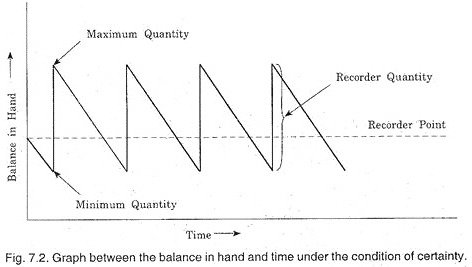
The cost of too large quantity consists of storage cost, interest on the money involved, and the risk of obsolescence. Now in min-max inventory control two points are to be known, i.e., reorder point and the quantity to be ordered. If there is no uncertainty, the graph between the time and balance on hand shows a pattern as shown in Fig. 7.2.
In this case, when the quantity on hand falls to the reorder point, an order must be placed for the ordered quantity. Since there is no uncertainty, this ordered quantity will arrive just as the stock at hand falls to minimum. Then with the new arrival the stock position reaches to maximum (i.e., minimum + ordered quantity = maximum). As consumption continues, the stock will again fall towards the reorder point.
ADVERTISEMENTS:
But under uncertainty, this is not the situation. As if no uncertainty is there, there is no need to maintain the minimum quantity, i.e., safe reserve at all, because the new order would arrive exactly on time, when inventory falls to zero. Now under uncertainty there are two types of uncertainty. Uncertainty about the rate of consumption of inventory and uncertainty about the amount of time required for delivering the new order.
The consumption increases with the demand and slows down in periods of declining in sales. The time required for supplying depends upon the supplier and on the transportation facilities—these are subjected to uncertainty. Further, if the parts stored are manufactured by the company itself, there is uncertainty due to the bottleneck in production, breakdown in machines and so on.
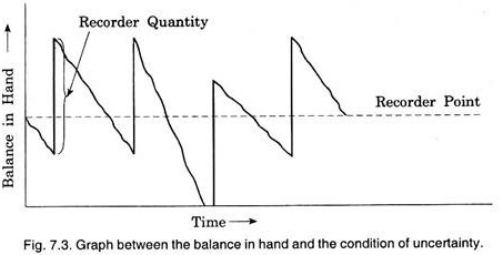
This is clear that min-max inventory control involves uncertainty, and to solve such problem the theory of probability is used. Now the pattern of graph (Fig. 7.2) changes to graph shown in Fig. 7.3.
The graph shown in Fig. 7.3 shows that the inventory will fall below the minimum, even down to the zero, because of rapid consumption or delay in the delivery or ordered quantity. Many times the inventory will reach above the maximum, because the slower consumption after the order was placed, or because of rapid delivery.
The consumption required for reorder point and ordered quantity is quite tedious and complicated which requires lengthy statistical procedures.


