4 Main Sections of Risk and Return Relationship

This article throws light upon the four main sections of risk and return relationship. The sections are: 1. Risk and Return of a Single Asset 2. Risk and Return of a Portfolio 3. Capital Asset Pricing Model (CAPM) 4. Arbitrage Pricing Theory.

Section # 1. Risk and Return of a Single Asset:

Return on Investment:

Return from a venture is concerned with benefit from that venture. In the field of finance in general and security analysis in particular, the term return is almost invariably associated with a percentage, and not a mere amount.

One of the major objectives of investment is to earn and maximize the return. Return on investment may be because of income, capital appreciation or a positive hedge against inflation. Income is either interest on bonds or debentures, dividend on equity or preference shares, etc.

Price change of the investment may lead to capital gain or loss. Hedge against inflation is a positive real rate of return. The expected return may differ from realized return.

The return of investment must refer to a particular period of time. Price change is the difference between the price at the end and the beginning of the period. Income may sometimes be nil and the price change can be both positive and negative or both can be positive and herein lies the risk. To generalize the return measurement as applicable to both fixed income security and variable income security is:

Total Return = Income received + Price change/Purchase price of asset

In security analysis, we are primarily concerned with returns from the investors’ perspective. Our main concern is to compute or estimate the return for an investor on a particular investment. The investment, one is concerned with, as a security analyst, is essentially a financial asset, say, a share or a debenture or some other financial instrument.

Rate of Return:

The rate of return on an investment for period (which is usually a period of one year) is defined as follows:

To illustrate, consider the following information about a certain equity share:

Price at the beginning of the year: Rs. 500

Dividend paid toward the end of year: Rs. 25

Price at the end of the year: Rs. 600

The rate of return on this share is calculated as follows:

25 + (600-500)/500 = 25%

It is helpful to split the rate of return into two components, viz. current yield and capital gains/losses yield as follows:

The rate of return of 25 percent in the example above may be broken down as follows:

25/500 + 600 – 500/500 = 5% Current yield + 20% Capital gains/loss yield

= 5 percent + 20 percent

Current yield + Capital gains yield

Risk and Uncertainty:

Meaning of Risk:

According to the Dictionary meaning existence of volatility in the occurrence of an expected incident is called risk. Higher the unpredictability greater is the risk. According to this definition risk may or may not involve money. All investments involve risk of one type or the other. People have many motives for investing in securities or assets.

But, the common man, while investing in securities has a very modest aim to earn a reasonably higher return on money. Risk and returns are two sides of the investment coin. Risk is associated with the possibility of not realizing return or realizing less return than expected. The degree of risk varies on the basis of the features of the assets, investment instruments, the mode of investment, the issuer of securities etc.

Even the so called risks less assets like bank deposits carry some element of risk. Thus, risk of an investment is the variance associated with its returns. The objective of risk management is not elimination of risk but proper assessment of the risk and deciding whether it is worth taking or not.

Risk and Uncertainty:

Some authors do not make any distinction between risk and uncertainty and use these terms interchangeably. Though risk and uncertainty go together, but they differ in perception. Risk refers to a situation where the decision maker knows the possible consequence of a decision and their related likelihoods.

Uncertainty involves a situation, about which the likelihood of possible outcome is not known. Uncertainty cannot be quantified whereas risk can be quantified of the likelihood of future outcomes. The degree of risk depends upon the features of assets, investment instruments, mode of investment etc.

Causes of Risks:

A number of factors which can cause risk in the investment arena are given below:-

i. Wrong method of investment

ii. Wrong Timing of investment

iii. Wrong quantity of investment

iv. Interest rate risk

v. Nature of investment instruments

vi. Nature of industry in which the company is operating

vii. Creditworthiness of the issuer

viii. Maturity period or length of investment

ix. Terms of lending

x. National and International factors

xi. Natural calamities etc.

Section # 2. Risk and Return of a Portfolio:

Portfolio analysis deals with the determination of future risk and return in holding various combinations of individual securities. The portfolio expected return is the weighted average of the expected returns, from each of the individual securities, with weights representing the proportionate share of the security in the total investment.

The portfolio expected variance, in contrast, can be something less than a weighted average of security variances. Therefore, an investor can sometimes reduce risk by adding another security with greater individual risk compared to any other individual security in the portfolio. This strange result occurs because risk depends greatly on the covariance among returns of individual securities.

Why does an investor has so many securities in his portfolio? If anyone security, let us say, security X, gives the maximum return, why not to invest all the funds in that security and thus, to maximise the returns? Answer to this query lies in risk attached to investments, objective of investment, safety, capital growth, liquidity and hedge against decline in the value of money etc.

The concept of diversification deals with this question. Diversification aims at reduction or even elimination of non- systematic risk and achieving the specific objectives of investors. An investor can even estimate his expected return and expected risk level of a given portfolio of assets from proper diversification.

Return on Portfolio:

From investors’ point of view, it is rarely advisable to invest the entire funds of an individual or an institution in a single security. Therefore, it is essential that each security be viewed in a portfolio context. Each security in a portfolio contributes returns in the proportion of its investment in security.

It is but natural that the expected return of a portfolio should depend on the expected return of each of the security contained in the portfolio. It is also important that amounts invested in each security should be logically decided.

Assuming that the investor puts his funds in five securities, the holding period return of the portfolio is described in the table given below:

The above table describes the simple calculation of the weighted average return of a portfolio for the holding period.

Risk on a Portfolio:

Risk on a portfolio is not the same as risk on individual securities. The risk on the portfolio is reflected in the variability of returns from zero to infinity. The expected return from portfolio depends on the probability of the returns and their weighted contribution to the risk of the portfolio. Two measures of risk are used in this context-the average (or mean) absolute deviation and the standard deviation.

The following table shows how the absolute deviation can be calculated:

First of all the expected return is determined in this case it is 15.00%. Next, all possible outcomes are analysed to determine the amount by which the value deviates from the expected amount. These figures shown in column 5 include both positive and negative values.

As shown in column 6, a weighted average using probabilities as weights will equal zero. To assess the risk the signs of deviations can be ignored column 7, shows the weighted average of the absolute values of the deviations, using the probabilities as weights, equal to 11%. This constitutes the First measure of likely deviation.

Another measure is standard deviation and variance. It is slightly more complex but preferably analytical measures. In this the deviations are squared, making all the values positive. Then the weighted average of these amounts is taken, using the probabilities as weights. The result is termed the variance. It is converted to the original units by taking the square root. The result is termed as the standard deviation.

Although both these measures are used interchangeably, the standard deviation is generally preferred for investment analysis. The reason is that the standard deviation of a portfolio can be determined from the standard deviation of the returns of its component securities, no matter what the distributions. No such relationship of comparable simplicity exists for the average absolute deviations.

We can think of a portfolio’s standard deviation as a good indicator of the risk of a portfolio, to the extent that if adding a Stock to the portfolio increases the portfolio’s standard deviation, the total stock adds risk to the portfolio. But the risk that the stock adds to the portfolio will depend not only on the stock’s total risk, its standard deviation, but on how that risk breaks down into diversifiable and non-diversifiable risk.

If an investor holds only one stock, there is no question of diversification and his risk is, therefore, the standard deviation of the stock. For a diversified investor, the risk of a stock is only that portion of the total risk that cannot be diversified away or its non-diversifiable risk. The non-diversifiable risk is generally measured by Beta (b) coefficient.

Beta measures the relative risk associated with any individual portfolio as measured in relation to the risk of the market portfolio. The market portfolio represents the most diversified portfolio of risky assets an investor can buy since it includes all risky assets.

This relative risk can be expressed as:

b = Non-diversifiable risk of asset or portfolio

Risk of market portfolio

Thus, Beta coefficient describes the relationship between the stock’s return and the market index return. A Beta of 1.0 indicates an asset of average risk. A Beta coefficient greater than 1.0 indicates above average risk and less than 1.0 indicates a below average risk.

One important point to be noted is that in the case of a market portfolio, all the diversification has been done, thus the risk of the portfolio is all non-diversifiable risk which cannot be avoided.

Similarly, so long as the asset’s returns are not perfectly positively correlated with the returns from other assets, there will still be some scope to diversify away its unsystematic risk. We can thus say that Beta depends upon only non-diversifiable risk.

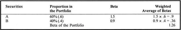
The Beta of a security portfolio is nothing but the weighted average of the Betas of the securities that constitute the portfolio, the weights being the proportions of investments in the respective securities as shown in the following table.

The systematic relationship between the return on the security or a portfolio and the return in the market can be described by using a simple linear regression identifying the return on a security or portfolio as the dependent variable and the return on market portfolio as the independent variable:

Thus X = α + BY + Er.

Where X = return on the security in the given period and Y is the market return.

α = The intercept where the regression line crosses the Y-axis.

B = The slope of the regression line.

Er = Error term containing all residuals

This equation can be explained with the help of the following diagram.

Diversification of Investments:

Risks involved in investment and portfolio management can be reduced through a technique called diversification. The traditional belief is that diversification means “Not putting all eggs in one basket.” Diversification helps in the reduction of unsystematic risk and promotes the optimisation of returns for a given level of risks in portfolio management.

Diversification may take any of the following forms:

i. Different Assets e.g. gold, bullion, real estate, government securities etc.

ii. Different Instruments e.g. Shares, Debentures, Bonds, etc.

iii. Different Industries e.g. Textiles, IT, Pharmaceuticals, etc.

iv. Different Companies e.g. New companies, new product company’s etc.

Proper diversification involves two or more companies/industries whose fortunes fluctuate independent of one another or in different directions. One single company/industry is always more risky than two companies/ industries.

Two company’s in textile industry are more risky than one company in textile and one in IT sector two companies/industries which are similar in nature of demand a market are more risky than two in dissimilar industries.

Some accepted methods of effecting diversification are as follows:

(i) Random Diversification:

Randomness is a statistical technique which involves placing of companies in any order and picking them up in random manner. The probability of choosing wrong companies will come down due to randomness and the probability of reducing risk will be more.

Some experts have suggested that diversification at random does not bring the expected return results. Diversification should, therefore, be related to industries which are not related to each other.

(ii) Optimum Number of Companies:

The investor should try to find the optimum number of companies in which to invest the money. If the number of companies is too small, risk cannot be reduced adequately and if the number of companies is too large, there will be diseconomies of scale. More supervision and monitoring will be required and analysis will be more difficult, which will increase the risk again.

(iii) Adequate Diversification:

An intelligent investor has to choose not only the optimum number of securities but the right kind of securities also. Otherwise, even if there are a large number of companies, the risk may not be reduced adequately if the companies are positively correlated with each other and the market. In such a case, all of them will move in the same direction and many risks will increase instead of being reduced.

(iv) Markowitz Diversification:

Markowitz theory is also based on diversification. According to this theory, the effects of one security purchase over the effects of the other security purchase are taken into consideration and then the results are evaluated.

Effects of Combining the Securities:

Holding more than one security in the portfolio is always less risky than putting all the eggs in one basket. As per Markowitz, given the return, risk can be reduced by diversification of investment into a number of scrips.

The risk of any two scrips is different from the risk of a group of two companies together. Thus, it is possible to reduce the risk of a portfolio by incorporating into it a security whose risk is greater than that of any of scrips held initially.

Example:

Given two scrips A and B, with B considerably less risky than A, a portfolio composed of some of A and some of B may be less risky than a portfolio composed of only less risky B.

Let

Expected Return – A – 40% – B – 30%

Risk (σ) of security – A – 15% – B – 10%

Coefficient of correlation, between A and B can have any of the three possibilities i.e. -1, 0.5 or + 1.

Let us assume, investment in A is 60% and in B 40%.

Return on Portfolio = (40 × 0.6) + (30 × 0.4) = 36%

Risk on Portfolio = (15 × 0.6) + (10 × 0.4) = 13%, which is normal risk.

Moreover, when two stocks are taken on portfolio and if they have negative correlation, the risk can be completely reduced, because the gain on one can offset the loss on the other. The effect of two securities can also be studied when one security is more risk as compared to the other security.

Interactive Risk through Covariance:

When individual securities are held by the investor, the risk involved is measured by standard deviation or variance. But when two securities are held in the portfolio, it is essential to study the covariance between the two. Covariance of the securities will help in finding out the interactive risk.

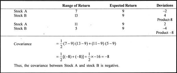
The covariance between securities is considered to be positive when the rates of return of the two securities move in the same direction. But if rates of return of the securities are independent, covariance is zero. If rates of return move in the opposite direction, the covariance is said to be negative.

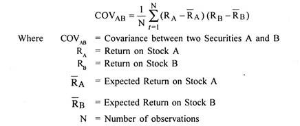
Mathematically the covariance, between two securities is calculated with the help of the following formula:

The probabilities remaining same and using the figures of the previous example of stocks A and B:

Coefficient of Correlation:

The coefficient of correlation is another measure designed to indicate the similarity or dissimilarity in the behaviour of two variables.

Taking the above mentioned stock A and B, coefficient of correlation can be calculated with the following formula:

Y_AB = COV_AB/σ_A σ_B

By putting the values given in the question we get:

Y_AB = -8/2×4 = -1.0

The coefficient of correlation between Stock A and Stock B is —1.0 which indicates that there is a perfect negative correlation and rates of return move in opposite direction. If Y is 1, then perfect positive correlation exists between securities and returns move in the same direction.

If Y is O, then it indicates that stocks’ returns are independent of each other. Thus, the correlation between two securities depends upon the covariance between the two securities and the standard deviation of each security.

Change in Portfolio Proportion:

If the amount of proportion of funds, invested in different stocks is changed e.g. in Stock A and Stock B, it will change the portfolio risk also.

Using the same example, the portfolio standard deviation is calculated for different proportions as follows:

Thus, by changing the investment proportions in different securities, the portfolio risk can be brought down to zero. If advantages of diversification are to be availed of coefficient of correlation has to be taken into consideration. This can be explained graphically also.

The graph proves that:

(i) The average risk of portfolio can be reduced if coefficient of correlation of the returns of Stock A and Stock B is less than 1.

(ii) If the coefficient is +1.0, the return moves along the straight line MN.

(iii) If the coefficient is —1.0, then, risk can be reduced to zero because the risk of one can be offset by that on the other.

(iv) When correlation is zero, securities at the curve provide better return than on the line.

Thus, if one is on the curve MN rather than on the straight line MN, one can increase the return without increasing the risk.

Example:

Stocks A and B displays the following parameters:

Solution:

The correlation is positive & very high. There is high degree of risk in combining the two securities.

Market and Non-Market Risk and Return:

The characteristic line procedure divides the security’s return into two components—one market related and one non-market related.

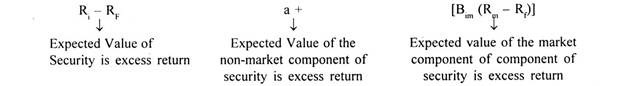
The non-market component of excess return is uncorrelated with the market component. The variance of the sum will thus equal the sum of the variance of the parts:

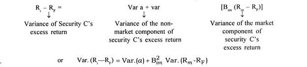
The risk of a security measured by variance can thus, be divided into two parts. One that is not related to market risk and one that is. Moreover, larger the latter, the more sensitive will be the security’s return to the market moves.

Section # 3. Capital Asset Pricing Model (CAPM):

William F. Sharpe developed the capital asset pricing model (CAPM). He emphasized that the risk factor in portfolio theory is a combination of two risks i.e. systematic risk and unsystematic risk. The systematic risk attached to each of the security is the same irrespective of any number of securities in the portfolio.

The total risk of portfolio is reduced with increase in the number of stocks, as a result of decrease in the unsystematic risk distributed over number of stocks in the portfolio.

A risk adverse investor prefers to invest in risk free securities. A small investor having few securities in his portfolio has greater risk. To reduce the unsystematic risk, he must build up a well-diversified portfolio of securities. A diversified and balanced portfolio of all securities will bring an investor’s risk in the stock market as a whole.

This is shown in the following figure:

Sharpe Asserts in CAPM that risky portfolios do not pay more than the safe ones. The systematic risk of two portfolios remains the same. To the rational investors, it makes no difference that the stocks in one portfolio are individually riskier than other stocks because successive stock price changes are identically distributed, independent of random variables.

An individual is assumed to rank alternatives in his order of preference. However, due to operating constraints e.g. limited finance he can avail only some of the alternatives. As such an individual chooses among the logically possible in the highest on his ranking. In other words an individual acts in a way in which he can maximize the return on his investment under conditions of risk and uncertainty.

Thus, the CAPM is a linear relationship in which the required rate of return K from an asset is determined by that asset’s systematic risk.

The CAPM is represented mathematically by the following equation:

K_n = R + [E(r_m)-R]b_n

Where b_n= Independent variable representing the systematic risk of the nth assets.

K = Dependent variable measuring the required rate of return.

The CAPM intersects the vertical axis at the risk less rate R, the quantity E(r_m) – R is the slope of the CAPM.

Capital Asset Pricing Model is represented by a CAPM line drawn on risk-return space. The CAPM relates a required rate of return to each level of systematic risk. The following figure portrays it graphically.

Point K represents the market portfolio and point R the risk less rate of return. Line RKZ represents the preferred investment strategies, showing alternative combinations of risk and return obtainable by combining the market portfolio with borrowing or lending.

The CAPM suggests a required rate of return that is made up of two separate components:

(i) The CAPM’s Intercept R represents the point of time. This component of the nth assets’ required rate of return compensates the investor for delaying consumption in order to invest.

(ii) The slope of the CAPM, E(r_m) – R, the second component is the market price of the risk. The market price of risk is multiplied by nth assets systematic risk coefficient. The product of this multiplication determines the appropriate risk premium i.e. Additional return. That should be added to the risk less rate to find the asset’s required rate of return. This risk premium induces investors to take risk.

Capital Market Line (CML):

The Capital Market Line (CML) defines the relationship between total risk and expected return for portfolios consisting of the risk free asset and the market portfolio. If all the investors hold the same risky portfolio, then in equilibrium it must be the market portfolio. CML generates a line on which efficient portfolios can lie.

Those which are not efficient will however lie below the line. It is worth mentioning here that CAPM risk return relationship is separate and distinct from risk return relationship of individual securities as represented by CML. An individual security’s expected return and systematic risk statistics should lie on the CAPM but below the CML.

In contrast the risk less end (R) statistics of all portfolios, even the inefficient ones should plot on the CAPM. The CML will never include all points, if efficient portfolios, inefficient portfolios and individual securities are placed together on one graph. The individual assets and the inefficient portfolios should plot as points below the CML because their total risk includes diversifiable risk.

Security Market Line (SML):

Security Market Line describes the expected return of all assets and portfolios of assets in the economy. The risk of any stock can be divided into systematic risk and Unsystematic risk. Beta (b) is the index of systematic risks. In case of portfolios involving complete diversification, where the unsystematic risk tends to zero, there is only systematic risk measured by Beta.

Thus, the dimensions of the security which concern us are expected return and Beta. The expected return on any asset or portfolio, whether it is efficient or not can be determined by SML by focusing on Beta of securities. The higher the Beta for any security the higher must be its equilibrium return.

Further the relationship between Beta and expected return is linear.

The SML expresses the basic theme of the CAPM i.e. expected rate of return increases linearly with risk, as measured by beta. It can be drawn as follows:

The SML is an upward sloping straight line with an intercept at the risk free return securities and passes through the market portfolio. The upward slope of the line indicates that greater expected returns accompany higher levels of Beta. In equilibrium each security or portfolio lies on the SML.

The above figure shows that the return expected from portfolio or investment is a combination of risk free return plus risk premium. An investor will come forward to take risk only if the return on investment also includes risk premium.

Thus the expected return on a portfolio E(R_m) consists of the following:

R_f = Risk free return (i)

R_m – R_f = Risk premium (ii)

R_m = Expected total return (1+2)

The CAPM has shown the risk and return relationship of a portfolio in the following formula:

E(R_i) =R_f + B_i (R_m-R_f)

Where E(R_i) = Expected rate of return on any individual security or portfolio of securities.

Rf = Risk free rate of return

Rm = Expected rate of return on market portfolio

B_i = Market sensitivity index of individual security or portfolio of securities.

Illustration:

Sunrise Holdings Ltd., an investment company has invested in equity shares of a blue chip company.

Risk free return (R_f) = 9%

Expected total return (R_m) = 16%

Market sensitivity index (B_i) = 0.8

Calculate the expected rate of return on the investment made in the security.

Solution:

E(Ri) = R_f + B_i (R_m – R_f)

= 9 + 0.8(16-9)

= 9 + 0.8(7)

= 9 + 5.6

= 14.6%

SML validates the claim that systematic risk is the only important ingredient in determining expected returns and that non-systematic risk plays no role. In other words, the investor gets rewarded for bearing systematic risk.

It is not total variance of returns that affects expected returns but only that part of variance in return that cannot be diversified away. If investors can eliminate all non-systematic risk through diversification there is no reason they should not be rewarded in terms of higher return for bearing it.

Limitations of CAPM:

Though the CAPM has been regarded as a useful tool for both analysts of financial securities and financial managers, it is not without critics.

The CAPM has serious limitations in the real world, discussed as follows:

(i) The CAPM is based on expectations about the future. Expectations cannot be observed but we do have access to actual returns. Hence empirical tests and data for practical use tend to be based almost exclusively on historical returns.

(ii) Beta (systematic risk) coefficient is unstable, varying from period to period depending up on the method of compilation. They may not be reflective of true risk involved. Due to the unstable nature of beta it may not reflect the future volatility of returns although it is based on the post history. Historical evidence of the tests of Beta showed that they are unstable and they are not good estimates of future risk.

(iii) CAPM focuses attention only on systematic (market related) risk. However, total risk has been found to be more relevant and both types of risk appear to be positively related to returns.

(iv) Investors do not seem to follow the postulation of CAPM and do not diversify in a planned manner.

(v) The analysis of SML is not applicable to the bond analysis, although bonds are a part of the portfolio of the investors. The factors influencing bonds in respect of risk and return are different and the risk of bonds is rated and known to investors.

Thus, it can said that the applicability of CAPM is broken by the less practical nature of this model as well as complexity and difficulty of dealing with beta values.

Risk Free Rate of Lending or Borrowing:

The three factors discussed in CAPM are systematic risk (B), the expected market return and the risk free rate. The risk free rate is the least discussed of the three factors. It is used only twice in CAPM. It is first used as a minimum rate of return (R) and it is used to find out the risk premium (r_m – R).

Thus, any error in estimating the risk free rate of return would lead to a wrong estimate of the expected rate of return for an asset or portfolio. Choosing a wrong risk free rate would mean that the analyst would misunderstand the sources of the asset’s returns, the quality of its performance or have poor data on which to make forecasts.

In CAPM theory, the risk free asset is one of the two choices available to the investor. The investor can reduce the risk of the portfolio by increasing the amount of risk free asset in the portfolio or he can increase the risk by reducing the risk free asset position or by borrowing at the risk free rate to further invest.

In fact, the risk free rate is the rate that will entice investors to choose between current or future consumption between savings or investment. The price required to induce an investor to forgo current consumption for a certain future sum, to forgo liquidity, is the price of time or the risk free rate of return.

The separation Theorem propounded by James Tobin States that the investors make portfolio choices solely on the basis of risk and return, separating that decision from all other characteristics of the securities. If particular assets are chosen on the basis of other factors, the CAPM is incomplete because it ignores other relevant factors.

Thus, it is implied that each investor will spread his funds among risky securities in the same relative proportion, adding risk free borrowing or lending in order to achieve a personally preferred overall combination of risk and return.

Risky portion of every investor’s portfolio is independent of the investor’s risk return preferences. The justification for this is that the risky portion of each investor’s portfolio is simply beyond the either axis.

Even if the investor commits zero proportion in these securities, the prices of these would eventually fall, thereby causing the expected returns of these securities to rise until the resulting tangency portfolio has a non-zero proportion associated with it. Ultimately, everything will be balanced out. When all the price adjusting stops the market will be brought into equilibrium.

Section # 4. Arbitrage Pricing Theory:

Like the CAPM, the Arbitrage Pricing Model is an equilibrium model of asset pricing, but its origins are significantly different. Whereas the CAPM is a single factor model, the APM is a multi-factor model. Instead of just a single beta value, there is a whole set of beta values-one for each factor.

Arbitrage Pricing Theory out of which APM arises states that the expected return on investment is dependent upon how that investment reacts to a set of individual macro-economic factors (the degree of reaction being measured by the betas) and the risk premium associated with each of those macro-economic factors. The APM was developed in 1976 by Ross.

This model does not depend critically on the notion of an underlying market portfolio. Instead, it is a model that derives returns from the properties of the process generating stock returns and employs arbitrage pricing theory to define equilibrium. Under certain circumstances it derives a risk return relationship identical to the SML of the CAPM.

The Arbitrage Theory is based on the following assumptions:

(i) The investors have homogeneous beliefs/expectations

(ii) The investors are risk avert utility maximisers

(iii) The markets are perfect so that factors like transaction costs are not relevant

(iv) The security returns are generated according to a factor model.

(v) Risk-returns analysis is not the basis.

The model takes the view that there are underlying factors that give rise to returns on stocks. Examples of these factors might include such variables as real economic growth and inflation or such financial variables as dividend yield and capital structure.

The objective of security analysis is to identify these factors in the economy and the sensitivities of security return to movements in these factors. A formal statement of such a relationship is termed as a factor model of security returns.

Single Factor Model:

According to this model the asset price depends on a single factor, say Gross National Product or Industrial production or interest rates, money supply, interest rates and so on.

In general, a single factor model can be represented in equation form as follows:

R = E + bf + e

Where E = Uncertain return on security I

b = Security’s sensitivity to change in the factor

f = the actual return on the factor

e = error term (unexplained variable)

Thus, this model only states that the actual return on a security equals the expected return plus sensitivity times factor movement plus residual risk.

Multiple Factor Model:

Empirical work suggests that a number of variables should be taken into account for asset pricing. The above mentioned equation can, thus be expanded to:

R = E + b₁f₁ + b₂f₂ + b₃f₃ + …………. + e

Each of the middle terms in the equation is the product of returns on a particular economic factor and the given stock’s sensitivity to that factor.

But the basic question is what are these factors? They are the underlying economic forces that are the primary influences on the stock market. Several factors appear to have been identified as being important. Some of these factors, such as inflation and money supply, industrial production and personal consumption do have aspects of being interrelated.

In particular, the researchers have identified the following factors:-

i. Changes in the level of industrial production in the economy

ii. Changes in the shape of the yield curve

iii. Changes in the default-risk premium (i.e. changes in the return required on bonds with different perceived risk of default.)

iv. Changes in the inflation rate

v. Changes in the real interest rate

vi. The level of personal consumption

vii. The level of money supply in the economy

Deriving the Arbitrage Pricing Theory:

With the help of APM, investment strategies of many types can be selected if there are many securities to be selected and a fixed amount to be invested the investor can choose in a manner that he can aim at zero non-factor risk. This is possible by combining securities to hedge out the sensitivity of a portfolio to all but one factor.

APT says nothing about either the magnitude or the rings of the factor coefficients or what the factors themselves might be. The model does not give us this guidance nor did Ross when he first found this model. The theory does not say anything about how the identity and magnitude of the factors should be determined.

It says that by active trading of securities with different sensitivities to the important factors, investors trade away opportunities for excessive gains. Since there are only a few systematic factors affecting returns, many portfolios are close substitutes for each other and thus will have the same value.

Excessive gains come only when, by buying some assets and selling others the investor hedges his portfolio and thereby insulates it from risk without eliminating excess return (the return above the risk free rate). These excessive gains are called arbitrage profits. In efficient markets, excess returns are eliminated by trading and investors cannot on average or over time, find opportunities to arbitrage for profits.

A simple example will demonstrate what arbitrage profit is and how an investor can take advantage of it; if it were available. Let us assume a market where there are only three assets, all sensitive to only one factor e.g. changes in the real interest rate: The sensitivities of each of the assets to the common factor, real interest rate and the expected returns are shown in the following table:

It can be seen that asset B is expected to have a return of 12%. Since the return that would usually be expected for an asset with sensitivity to interest rate is 10.5%, asset B promises an excess return of 1.5%.

To take advantage of this excess return and to do so with no risk, an investor can arbitrage among three assets; the investor with Rs. 2000 need only buy Rs. 1000 of asset B and short sell Rs. 667 of risk free security A and Rs. 333 of security c.

The results of buying and short selling activities are shown in the following table:

The investors earns 1.5% excess return and do so without risk, the factor sensitivity of asset B is offset by the average sensitivity of the short sold portfolio. Inequities offer opportunities to arbitrage.

The same situation exists when assets are priced on more than one factor. APT allows for as many factors as are important in the pricing of the assets. The APT thus describes the behaviour of most investors, who are opportunity seekers and believe that opportunities to make profits exist.

Such investors however dislike higher levels of risk. The fact is that there is always a trade-off between risk and return, which is not considered by the APT model. Therefore, in practical portfolio operations, it is better to combine the Capital Asset Pricing Theory and the APT model.