Mathematical Analysis of Investment Project | Firm | Management

In this article we will discuss about the mathematical analysis of firm’s capital investment project.  

The net present value of a project is equal to the sum of the present value of all the cash flows (inflows and outflows) associated with the project.

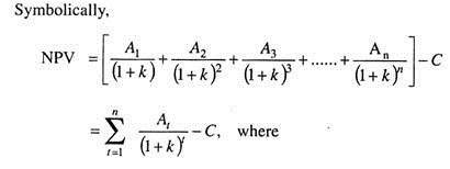
NPV = Net present value,

A_n = Cash flow occurring at the end of the year t (t = 1,……. n). A cash inflow has a positive sign, whereas a cash outflow has a negative sign.

n = Life of the investment project.

k = Cost of capital used as the discount rate (also termed as risk-free interest rate).

C = Cost of investment/project proposal.

The ‘Net Present Value’ has considerable merits:

(i) It takes into account the time value of money.

(ii) It considers cash flow stream in its entirety.

(iii) It represents the contribution to the wealth of shareholders.

(iv) It can be used to select between mutually exclusive projects.

(v) It assists in ranking the projects in order of net present values—that is, a project with highest positive NPV is adjudged first rank and so on.

The basic feature of NPV is: it is based on the assumption that intermediate cash inflows of the project are re-invested at a rate of return equal to the firm’s cost of capital.

The limitations of NPV are:

(i) The ranking of projects on the NPV dimension is influenced by the discount rate (or risk-free interest rate), and

(ii) The alternative with higher NPV may involve larger economic life to the point that it would be less desirable than an alternative having a shorter life.

Background Note about ‘Standard Deviation of NPV (This does not form part of the answer):

The Standard Deviation is an absolute measure of risk. It measures the deviation of a variable between its possible value and arithmetic mean, duly weighted by probability associated with the possible values. Symbolically,

 

 

Where

σ= standard deviation

p_i = probability associated with the i th possible value

R_i = i th possible value of the variable

r = arithmetic mean of the variable

The square of the standard deviation, σ² is called variance.

For risk analysis, an expert usually thinks about the dispersion of cash flows (that is, the difference between the probable cash flows that can occur and their expected values). This dispersion of cash flow is indicative of risk. In this sense, standard deviation measures the variance about the expected cash flows of each of the probable cash flows. Standard deviation is most commonly used in financial analysis.]

In mathematical analysis, the concepts of expected NPV and the standard deviation of NPV are of great importance.

For mathematical analysis, the nature of cash flows may be looked into from three aspects:

(i) No correlation among cash flows,

(ii) Perfect correlation among cash flows, and

(iii) Moderate correlation among cash flows.

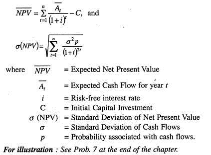
Un-correlated Cash Flows:

There is no relationship between cash flows from one period to another.

In this case, the expected NPV and the standard deviation of NPV are expressed by the following formulae:

Perfectly Correlated Cash Flows:

In this case, the cash flows of all years are linearly related to one another.

The formu­lae are:

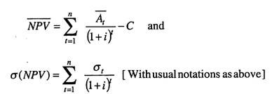
and the mean (A_t ) and standard deviation ((σ_t) of cash flows are considered by the strategist.

Moderately Correlated Cash Flows:

These cash flows do not conform to either of the above patterns—independence and perfect correlation, discussed before. These cash flows are needed to be evaluated with the help of a series of conditional probabilities.

In this case, the project is assumed to generate year-wise cash flows depending on the demand levels (high or low). For example: in year 1, there may be two cash flows with probability factors for two possible levels of demand; similarly, in year 2 there may be two cash flows with probabilities for two demand levels, and the same pattern in year 3 and so on.

The probabilities in year 4 are called initial probabilities and those in subsequent years (say, year 2 or year 3, etc.) are termed conditional probabilities because the cash flows in subsequent years are dependent upon what happened in earlier years (that is, in years 1 and 2 in case of 3 years being considered).

In such case:

(i) Net cash flows, year-wise, are arranged to form a cash flow stream; and

(ii) Probabilities (associated with cash flows), year-wise are converted to have joint probabilities which are obtained/determined by mere multiplication process [for example: if the year-wise probabilities are 0.5, 0.8 and 0.6, then joint probability is (0.5) x (0.8) x (0.6) = 0.240].

The procedure to compute the net present value is almost the same as outlined before. The system is as follows:

(i) Discounting the cash flow of each series by the risk-free interest rate to get present values;

(ii) Finding out the sum of stream-wise present values;

(iii) Multiplying the sum (at ii) by joint probability to arrive at expected values;

(iv) Finding out the sum of all expected values and subtracting there from the initial cost of the project to obtain the expected net present value (NPV).

To determine the standard deviation of the net present value, the following formula is used:

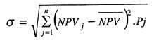
where NPV_j is the net present value for series j of net cash flows, covering all years, NPV is the expected value of net present value of the project and P. is the probability of occurrence of that series.

Comment:

The strategist, while applying mathematical analysis for project evaluation, should bear in mind the following:

1. The degree of correlation among cash flows should be correctly determined to measure the risk.

2. The risk of a project will be significantly high when cash flows are perfectly correlated than when they are independent.

3. If the degree of correlation is wrongly estimated, then it leads to use of a wrong formula to measure the risk—which ultimately leads to the incorrect accept-reject decision.