Essay on Network Analysis | Production Planning | Production Management

Read this essay to learn about the two main methods and techniques used for network analysis in an organisation. The techniques are:- 1. Critical Path Method (CPM) 2. Project Evaluation Review Technique (PERT).

Essay  # 1. Critical Path Method of Network Analysis:

It is observed that in a network one can enumerate man sequences of activities from starting event to end event. Each sequence will contain different combination of activities with different duration. One of the important object to network analysis is to know the minimum possible time by which the project can be completed. This is done by determining the cortical path i.e. the sequence of activities with longest duration.

It is known as critical path because any delay in activities lying on this path would cause a delay in the whole project. To quicken the process, the activities lying on the critical path should be taken first.

The activities lying no Non-critical path have some flexibility in their starting time and their extension or delay in start is not likely to affect the final completion date. These are known as Stack activities and should be given priority in order of their float value.

Development of Critical Path Method (CPM) has provided a basis for more formal and general approach towards project management. This technique can be used in situations where duration of various activities can be accurately visualised from path experience, CPM provides interrelationship among the elements of the project and identifies the relative importance of each element in the overall schedule.

CPM methods can be applied with notable success to large-scale research and development programmes e.g. construction work, industrial maintenance and installation operations.

Critical path method (CPM) is an effective tool of scheduling and planning. This also overcomes the limitations of Gantt chart. By CPM, one can understand that how the activities and operations of a project fit with each other and the logic of the proposed solution can tested.

Following are the main objectives of CPM analysis:

(i) To determine a route between two or more operations which optimizes some measure of performance.

(ii) To locate this obstacles and difficulties involved in a production process.

(iii) To assign the starting and finishing times for each operation or activity.

(iv) To determine the float associated with each non-critical activity.

The enumeration of total duration for each sequence of activities for a real life project is very difficult to calculate. But if some systematic procedure is adopted then the complications in the enumeration process can be reduced to manageable proportions. This can be done by the calculation of various time estimates associated with each operation. For the determination of critical path two kinds of time estimates are calculate.

Time Estimates to Find the Critical Path:

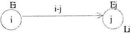
The time estimates for any event in a network are calculated in context with the proceeding and the succeeding activities for that event. Any event does not consume any time or resource. It merely indicates the start of the subsequent activity and the end of the proceeding activity.

Earliest Start Time (EST):

It is the earliest possible time for an event to indicate the start of an activity. If only one activity converges towards the event, then, the EST of the event can be calculated by the EST of the event at the tail of the activity plus the duration of the activity.

 

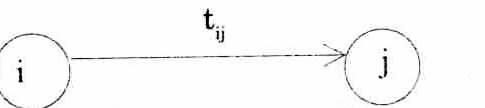
EST for event (i) = EST fpr (i) + tij

In case more than one activities are merging towards an event then the following rule is adopted.

Calculate EST’s for the event under consideration by considering the EST at the tall events of all activities plus the time duration of each activity and select the highest value from all these EST’s pf the event.

The concept is based on the fact that no event can be considered to be reached unless all the activities proceeding to it are completed.

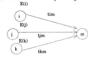
EST (m)I from activity i-m = Ei + tim

EST (m)j from activity j-m = ej + tjm

EST (m)k from activity k-m = Ek + tkm

The maximum of EST (m) I, EST (m)j and EST (m)k will be E(m). For the calculation of EST we proceed from left to right in a network.

Latest Finish Time (LFT):

It is the latest time by which an event should finish otherwise the activity subsequent to the event will be a delayed. It is calculated by the LFT of the event at the head of the subsequent activity minus the duration of that activity.

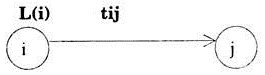
If there are more than one subsequent bursting from event (i), then compute L (i) Via all the paths that emanate from I and choose the smallest value as L(i).

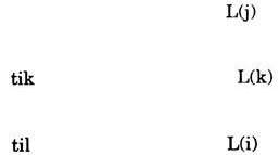
L(i) = L(j)-tij

L(i)k =L (k)-t jk

L(i)j = L(i)-til

Smallest calculation L(i)j, L(i)k and L(i)l will be taken as L(I).

For the calculation of LFT we proceed from right to left in a network.

Est and LFT for starting event are always zero and EST and LFT for the end event are always same.

Method for calculating EST and LFT is illustrated by example 1.

Example 1:

Calculate EST and LFT for the network given in Fig. 8.6:

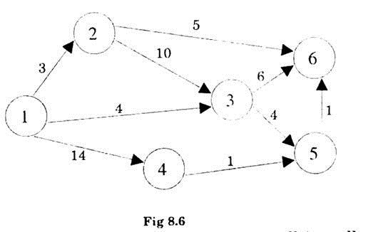
Solution:

Any activity can start only when all its tall end events are completed. The EST of starting event is always taken to be zero. So EST for event (1) is zero.

Event 2 can start when the activity before it is complete. The duration of that activity is 3 units, hence EST for event2

EST (2) = EST of event 1 + duration of activity-preceding to event2 = 0 + 3 = 3 time units.

Similarly EST of event 4

EST (4) = EST of event (1)+duration of activity before event 4 = 0 + 14 = 14

Now for event 3 there are two activities preceding to it and emerging from the events 1 and 2. Thus EST for 3 can be either.

EST of 1 + duration of activity emerging from 1 i.e. (1-3) = 0 + 0 = 4

Or EST of 2 + duration of activity emerging from 2 i.e. (2-3) = 3 + 10 = 13

But all activities before event 3 should be completed before the start of event (3). Hence maximum of 4 and 13 will be the starting time of 3. Thus EST for 3 will be 13.

Similarly there are two events preceding to event 5 i.e. event (3) and event

4 So EST of 45 can be maximum of:

(i) EST of (3) + duration of activity3-5 = 13 + 4 = 17

(ii) EST of (4) +duration of activity4-5 = 14 + 1 = 15

Hence EST of (5) = 17

Now for event (6) there are three events preceding to it, namely events 2, 3 and 5.

The EST of 6 can be maximum of:

(i) EST 2  + duration of activity 2-6 = 3 + 5 = 8

(ii) EST3 + duration of activity 3-6 = 13 + 6 = 19

(iii) EST 5 + duration of activity 5-6 = 17 + 1 = 1

Hence EST of 6 will be 19 time units. LET for 6 will also be 19.

Thus the total duration of the project is 19 time units.

Latest finishing time can be calculated by moving for right to left for each event in the network and subtracting the duration of activities from the LFT of the Head event of that path e.g. for event(5) LFT (5) = LFT (6) – duration of activity 5-6 = 19-1 = 18

LFT (4) = LFT (5)-duration of activity (4-5) = 18-1 = 17

But for event 3 there are two paths for consideration namely 3-5 and 3-6.

The minimum of these times will be taken as LFT (3) i.e.

LFT (6)-duration of activity (3-6) = 19-6 = 13 units.

AND LFT (5) – duration of activity (3-5) = 18-4 = 14

Minimum of 13 and 14 i.e. 13 will be LFT for 3.

Similarly LFT pf 2 will be minimum of

(i) LFT (6)-duration of activity (2-6) = 19-5 = 14

(ii) LFT (3)-duration of activity (2-3) = 13-10 = 3

i.e. LFT of 2 = 3 units.

LFT of event (1) will be same as its EST i.e. 0.

Thus EST and LFT for the various events are

 

 

 

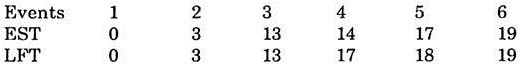
The above procedure of calculating EST and LFT appears to be quite complicated and cumbersome. Alternately these estimates can be calculated by MATRIX method.

Matrix Method for EST and LFT:

The procedure appears to be simple and straightforward with lesser chances of committing error in calculation of EST and LFT. Here a square with rows and columns equal to (number or event in the network +2) is drawn e.g. in example 1 there are six events, so we will draw a square with 6 + 2 = 8 rows and 8 columns. Inscribe EST in 1^st row and 1^st column and LFT in the last row and first column of the square. Also draw a diagonal across the second column of first row and last column of last but one row.

The event numbers are written from 3^rd to the last columns of first row and the second row to last but one row of second column. Duration of each activity in entered in a cell for which the row corresponds to tail event and column corresponds to head event of the activity.

Thus for Example 1 we shall get the matrix given in fig.8.7. e.g. in network of fig. 8.4. duration of activity 3-5 is 4 units. So in the matrix we write 4. In the same way duration for other activities is inserted in corresponding cells of the matrix.

Computation of EST:

EST corresponding to event (1) is taken as zero. Now for event (2) proceed in row for event two from left to right till we reach the column for event (2) and locate the time estimates above the diagonal in column for event (2). Here there is only one time value i.e.3. So add this to the EST in the corresponding row. Thus EST for event two becomes 3. Now for event (3) proceed in the same way as for event (2) and locate the time estimates just above the diagonal in column for event (3).There are two time values namely 4 and 10. Add these values to the EST in the corresponding rows i.e.

For time 4                 4 + 0 = 4

For time 15              10 + 3 + 13

And taken maximum of these i.e. 13 as EST for event (3).

Continue the process till EST for all events are calculated.

Latest Finish Times (LFT):

LFT for event 6 is equal its EST. So enter 19 in the last column of last row in the matrix.

Now move to the column for event 5 and find the times along the diagonal. There is only one value i.e. 1. Subtract it from the corresponding LFT i.e. 19 to get LFT for event 5. Thus LFT for event five is 19 – 1 = 18 and is entered in the column for event 5 in last row of the matrix.

Then move to the column 4 and see the number of time values across the diagonal in row for event 4. There is only one value i.e. 1. lying in the fifth column. Subtracting 1 from LFT for event 5 i.e. 18, we get LFT for event 4 as 18 – 1 = 17. Enter it in last row of column corresponding to event 4.

Now in row for event 3, there are two values 4 and 6 across the diagonals in columns for 5^th and 6^th events. Subtract these times from the corresponding LFT’s and select the minimum as LFT for event3. i.e.

(i) LFT for event (5) – 4 = 18 – 4 = 14.

(ii) LFT for event (6) – 6 = 19 – 6 = 13

So 13 is LFT for event 3 and is entered in last row of column for event3. Similarly we can calculate LFT’s for events 2 and 1. Matrix method is a more ordered and systematic procedure for calculating EST and LFT. But this method is workable only when the number of events does not become too large.

Critical Path from Time Estimates:

The critical path connects all those events for which EST and LFT are same. The difference between LFT and EST is known as stack of the event. So critical path events have zero stack. This implies that as soon the preceding activity for any events is over the subsequent activity has to start; otherwise the project will be delayed. Thus all activities lying on the critical path cannot be adjusted w.r.t. to start or finish times.

In example 1 EST for events 1, 2, 3 and 6 are same. Hence the critical path is

1      2      3      6 with a duration of 19 time units

CPM can be Effectively used in the Following Situations:

(i) Location or, and deliveries from a warehouse.

(ii) Production planning.

(iii) Communication Networks.

Time Estimates Associated with Activities of a NETWORK:

There can be four kinds of time estimates associated with activities of a NETWORK. These time estimates can be used to analyse the network or appropriate resource allocation.

The time estimates are:

(i) Earliest Start Time(EST):

It is the EST of the event from , which the activity arrow originates.

EST for activity i-j will be L(j)

(ii) Latest Finish Times (LFT):

It is the LFT of the event at which the activity are terminates, i.e. LFT for I-j will be L(j).

(iii) Earliest Finish Times (EFT):

This is the sum of EST of the activity and its duration i.e. EFT of I-j = EST + tij

(iv) Latest- Start Time (LST):

This is the difference between the LFT of the activity and its duration i.e. EST(I-j) = LFT-tij

The total duration of the time available for any activity is the difference between its EST and LFT.

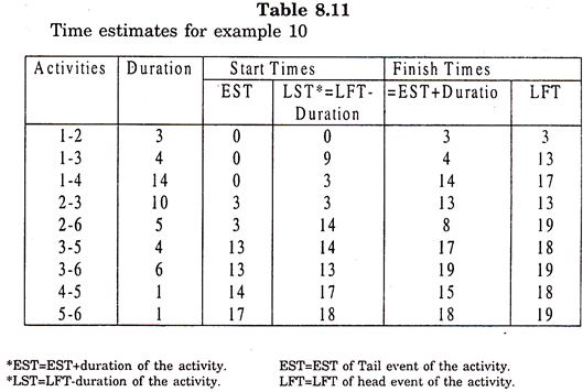
The Table 8.11 gives the time estimates of various activities for the network of Example 1.

Time estimates for example 1:

 

Concept of Floats and Slack:

Slack:

It is the freedom for scheduling or to start any event. It is always associated with an event and is calculated by its EST and LFT, An event for which the slack time is zero is called critical event.

The critical path is located by all those events for which stack time is zero.

Floats:

The maximum amount by which the duration of an activity can be increased without increasing the total duration of the entire project is known as Total Float.

Presence of float in a project signifies under utilisation of the resources and indicates the points of inherent flexibility in the process. There are three kinds of Float namely, Total float, Free float and independent float.

Total Float = [LFT of Head event – EST of tail event] – duration of the activity

Total Float for (i – j) = [LFT(j) – EST(i)] – duration (i – j)

= [LFT (j) – duration (i – j) – EST (i)]

= LST(i) – EST (i)

The value of Total float provides following information about the process.

Free Float:

It is that time by which an activity can be rescheduled without affecting the succeeding activity i.e.

Free Float = Total Float-Slack time of Head event, i.e. Free Float for (i-j)

= Total Float-Slack time for event (j)

Independent Float:

The time by which an activity can be rescheduled without affecting both preceding and succeeding activities is known as independent float i.e.

Independent Float = Free Float-stack time of tail event i.e. Independent Float for (i – j) = Free Float (i-j)-slack for event i.

It should be remembered that slack is always associated with events and Float with activities.

The method of calculation of floats is illustrated for example 1.

The floats associated with various activities in Network of fig. 8.6. can be calculated with the help of time estimates in Table 8.11 and are presented in Table 8.12.

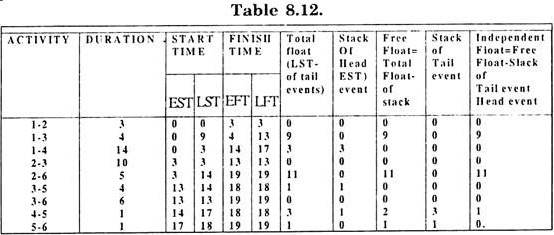
e.g. Total Float for activity (4 – 5)

= [LFT of head event i.e. 5-EST of tail event i.e. 4] – duration of the activity = (18 — 14) — 1 = 3

Which is same as LST of tail event – EST of tail event = 17 – 14 = 3

Free Float = Total Float-Slack of Head event i.e. 1. = 3 – 1= – 2

Independent Float = Free float- stack of tail event = 2 – 3 = – 1

Example 2:

A project schedule has the following characteristics:

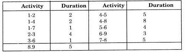
Construct a network and find critical path, total duration of the project and various time estimates.

Solution:

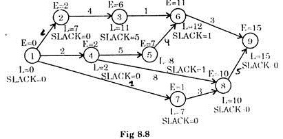
Fig 8.8 gives the required network for the given problem.

Calculation of Floats and Time Estimates.

Following the method described in Ex. 1, the time estimates are calculated first moving from left to right and then from right to left. These estimates for various events are shown on the events in fig 8.8.

Now the critical path consists of all those events for which EST = LFT.

Thus critical path for the problem is

1    →    4    →    8    →    9

With a duration of 15 time units.

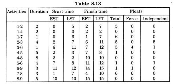
The various time estimates and Floats are calculated in Table 8.13.

Here EFT = EST + duration of activity

LST = LFT – duration of activity

For Floats, slack of the events can be seen from fig 8.8.

Essay # 2. Project Evaluation Review Technique (PERT) of Network Analysis:

CPM and PERT are modern techniques of Network Analysis for planning and control of big project in areas of Chemical, Defence, Building Construction and other industries. Here the project to be planned is broken into interdependent activities and a network is constructed to depict these relationships. PERT is similar to CPM.

But, CPM can only be applied when the duration of each activity can be determined accurately from experience or from past records/work study methods.

In present environment, because of various uncertainties involved in a system, extract duration of each activity is very difficult to determine. In such situation where some sort of uncertainty is associated with time such situations where some sort of uncertainly is associated with time estimates of various activities CPM cannot be used but PERT can be applied.

PERT also provides the confidence limits for the expected duration of the project. The basic difference in the methodology of CPM and PERT is that CPM gives more importance to the activities whereas PERT lays more emphasis on events.

Features of PERT:

(i) Draw the network for the project.

(ii) Three time estimates namely optimistic, normal and pessimistic times are estimated for each activity to take into account the presence of uncertainties

Optimistic Time t₁:

The shortest possible time to complete and activity without any provision for any delay or set-backs.

Normal Time t₂:

This is the time most often required to perform an activity, Here it is assumed that the situation is almost normal with few set-backs or leps.

Pessimistic Time t₃:

It is the longest time for the accomplishment of an activity under adverse conditions. This time corresponds to abnormal situations where everything has gone wrong e.g. major calamities like labour strikes; acts of God etc. are excluded from consideration. This time is very difficult to determine.

(iii) The three time estimates are used to calculate the expected time for each activity.

(iv) Critical path and stack time are computed. The sequence of activities which has maximum expected time for the completion of the project determines the critical path.

(v) The three time estimates are provided by a person who is in-charge of the operation and the values are generally based on his judgement and experience.

(vi) The time estimates are assumed to follow a Beta distribution.

The assumption of the Beta distribution, however, is not flawless and the calculations made on this assumption may, sometimes, be in error to the tune of 30%.

Probability Distribution:

The distribution of times associated with activities in a production process is found to be a BETA distribution with

The probability distribution can be used to find the probability that the project is completed on some desired date.

The expected E(t) for the completion of a project and the corresponding variance V(t) implies that if the whole project is repeated a number of times under identical conditions then the average duration of the project will be equal to E(t).

The information can be used to calculate the probability that the project will be completed within a desired time say D. Here we assume the distribution for the total duration of the project to be normal. Then the standard normal variate for time D is given by

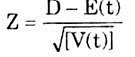
Now with the knowledge of average and standard deviation the probability of work being completed by some stipulated time can be derived.

The required probability for given Z can be calculated from standard table of normal distribution. Method is illustrated by the Example 3.

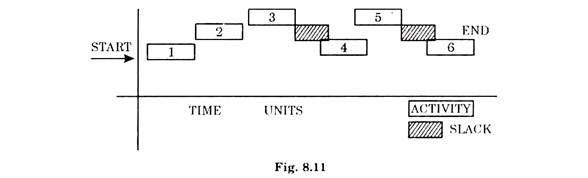
A typical PERT diagram is shown in fig 8.11.

Example 3:

The following table gives the activities in a construction project and other relevant information:

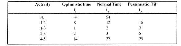
(i) Draw a PERT diagram.

(ii) Find probability that the project will be completed in les than 60 days.

Solution:

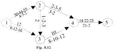
The PERT network is drawn in fig 8.12.

The best estimated time for each activity and the corresponding variance is calculated on the assumption that the distribution of time in the production process is Beta.

Thus using the formulae

Best estimated time to = t₁ + 4t₂ + t₃/6

and variance of the estimate = (t₃ – t₁/6)²

we get the time estimate in table 8.17.

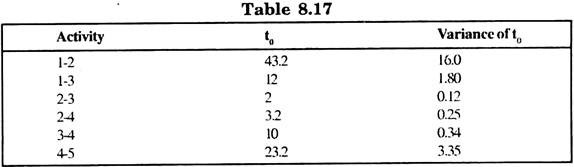
Using the best estimated times, we can calculate the critical path, which comes out to be: 

1     →     2     →     3     →     4     →     5

With an estimated time of the project = {43.2 + 2 + 21.2} = 76.5 days.

With variance = 16.0 + 0.12 + 0.45 + 3.35 = 19.92

The confidence limits for the completion time of the project are given by: 

76.5 ± 1.96 x √(19.92) i.e. 85 and 68 days approximately

The Calculation of probability can be done with the help of normal distribution shown in fig 8.13.

Here due date = 60 days

E(t) = 76.5 days

and V (t) = 19.92

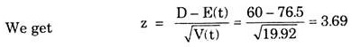
From the tables of normal distribution, we find the required probability i,e.

P (Z ≤ 3.69) = 0.011 approximately; which is very small

Limitations of PERT are:

(i) Expected time and the variances are only approximate values which may not be true in many situations.

(ii) The assumption of 3 distributions is difficult to be valid in practice.

Time-Cost Trade off in Network:

CPM/PERT in a network determines that sequence of activities which requires maximum normal time for the completion of the work i.e. with the available resources the operation of the events/ activities lying on the critical path cannot be performed in less than the required time. But very organisation wants to reduce the target time so that the surplus/saved time can be used for extra work by sending extra resources.

Further more, every enterprise wants to accomplish the desired objective at minimum cost also. Sometimes it may be desirable to extend the project duration if there is considerable saving in costs. Thus time- cost relationship is of great significance in project management.

The project cost consist of both direct and indirect costs, direct costs are related with the duration of the activities and include costs on inputs to perform that activity. Indirect costs include overhead costs, the specified date.

The duration of the project can be shortened by systematic analysis of Critical Path activities, crashing costs and corresponding costs and corresponding affect of indirect costs. For this time-cost relationship should be critically examined.

The relationship can be studied with the help of the following costs and time values:

(i) Normal Time:

The time associated with normal resources of the organisation to perform the activity is known as normal time.

(ii) Normal Cost:

The expenditure incurred on normal resources for completing any activity in normal time is known as normal cost.

(iii) Crash Time:

The reduced time for the completion of any activity by using additional resources is known as crash time.

(iv) Crash Cost:

The total expenditure incurred on normal and additional resources for cashing the time is known as crashed cost.

The behaviour of normal and crashed cost/ time is illustrated in fig. (8.14).

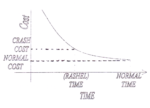
Actual time-cost relationship could be of any shape butt with the assumption of linearity of time-cost trade-off for an individual activity, the cost stop in defined as

Cost Slope = Crashed cost-Normal Cost/Normal Time-crashed Time

Cost slope represents the extra cost of shortening the duration of the activity by one time unit. For reducing the activity duration the management may agree for extra expenditure but to keep this expenditure minimum we must concentrate only on those activities for which cost slope is minimum.

The time-cost trade off method consists of systematic analysis of project cost and time. If can be observed that shortening the duration leads to increase in direct costs but decrease in indirect costs and the strategy will be justified only when it results in net saving.

The normal tendency of every manufacture is to produce at minimum cost and to have most efficient use of the resources. But in emergencies or sudden rush of orders if production is to be increased by increasing rate of production then naturally additional resources are to be introduced which will result in additional expenditure. Manufacture will be tempted to crash the time only when the profit earned from additional production is more than the extra expenditure on crashing.

Besides expenditure on resources to perform various activities involved in a production process there are some Indirect Costs involved in cost of production namely administrative costs, building maintenance costs, other overheads and penalty for delay, if any, some organisations pay bonus to workers for efficiency.

The expenditure incurred on performing various activities is known as direct cost.

The production/project cost is the sum of direct and indirect costs.

The following are the steps in time-cost trade off method:

(i) Jobs are assigned at their EST with normal resources to have maximum length schedule.

(ii) Identify those activities lying on the critical path whose cost slopes are less than the indirect costs.

(iii) To reduce the project duration, one or more of the activities on critical path are expedited at added cost.

(iv) If the reduction in time in step (ii) results saving in indirect costs and this saving is more than additional cost incurred in step (ii) then the new schedule will be less expensive.

(v) New schedules are generated as long as the activities can be crashed and there is reduction in total costs.

(vi) If at any stage there are some parallel critical paths then one job/activity in each of them must be chosen for crashing.

The estimation of crashed cost and crashed time is explained by example 4.

Example 4:

A marketing manager wants to launch a new product. The network of the activity is given in Fig. 8.15.

 

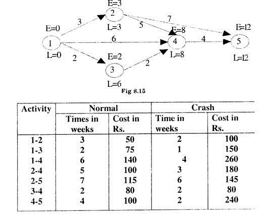
The crash is the minimum feasible time for executing the activity, using maximum feasible resources. Suppose the indirect costs are Rs. 900 per week. Find the project cost trade off.

Solution:

First of all critical path is determined by calculating EST and LFT for various events by the method explained in example 1. The time estimates are shown on the network of fig. 8.10.

Critical path is determined by all those events for which EST = LFT.

Here critical path will be 1     →     2     →     3     →     4     → 5 with a duration of 12 weeks.

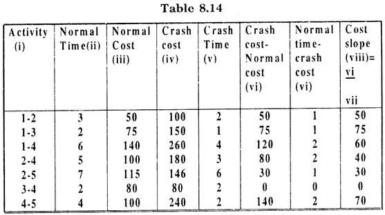
For time crashing, we calculate the crash cost/week for each activity i.e. the cost slope. These are given in Table 8.14.

Now for time crashing we consider possible paths in the network and the corresponding durations in the table 8.15.

The first step in time crashing is to identify these activities along the critical path whose costs slopes are less than the indirect cost. Take these activities in order of increasing cost slopes.

In this example all cost slopes are less than the indirect cost. Now we consider the activities on critical path in order of the cost slopes for crashing. All other paths are also considered simultaneously to see whether crashing is affecting the change in critical path at any stage of crashing or not.

The systematic calculations can be done in the following tabular form (see table 8.15).

The activities on critical path in order of their cost slopes are (2 – 4), (1 – 2) and (4 – 5).

So we first consider the activity 2-4 with minimum cost slope for crashing. The activity can be crashed by a maximum of 2 weeks.

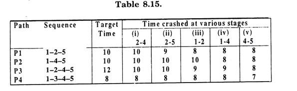
(i) So reducing the time of activity 2 → 4 by two weeks at a crush cost of Rs. 40, the target time becomes 10 for P3 and at this stage P3 still remains as critical path.

(ii) Now the activities lying on paths PI, P2 and P3 in increasing order of cost slope are 2-5, 1-2, 1-4 and 4-5. Thus crashing 2-5 by one week we get duration of PI as 9 weeks. At this stage P2 and P3 become the critical paths.

(iii) The next activity in order of cost slope is 1-2 with a possible crash of one week. At this stage path P2 is the critical path with a duration of 10 weeks. This duration of PI cannot be crashed further.

(iv) For P2 the activity with minimum cost slope of 60 is 1-4 with a possible crash by one week. After this P2 and P3 are further crashed by one week for the activity 4-5.

It is observed that further reduction in the target time is not possible as there is no further scope of reducing the time of any critical path.

T: Crashed cost can be calculated in the following tabular form (Table 8.16):

Thus the total crashed cost = Normal expenditure + expenditure on crashing + indirect costs.

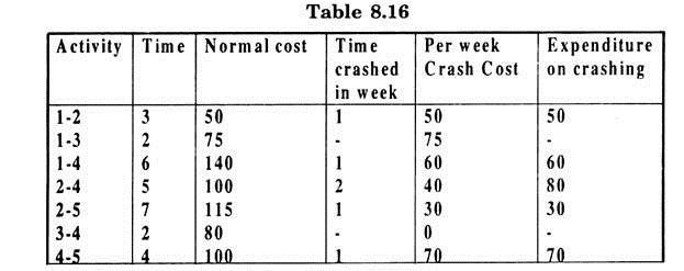
= Rs. 660 + Rs. 290 + Rs.(8 × 900)

= Rs. 660 + Rs. 290 + Rs. 7200

= Rs. 8150

With crashed time of 8 weeks.

It can be observed that contraction in time has resulted in reducing the overall cost also. The reduction of weeks has been achieved by an expenditure of Rs. 290 only, where the indirect cost has been reduced by Rs 3600. The problem illustrates the value of a network in management planning and time scheduling.