
This article throws light upon the top two techniques used for adjusting time value of money. The techniques are: 1. Compounding Technique 2. Present Value Techniques.
Adjusting Time Value of Money: Technique # 1.
Compounding Technique:
The time preference for money encourages a person to receive the money at present instead of waiting for future. But he may like to wait if he is duly compensated for the waiting time by way of ensuring more money in future.
For example, a person being offered Rs. 100 today may wait for a year if he is ensured of Rs. 110 at the end of one year (taking his preference for an interest of 10% p.a.) The cash flow of Rs. 100 at present or Rs. 110 after one year will be the same for this person.
ADVERTISEMENTS:
The future value at the end of period I can be calculated by a simple formula given below:
V1 = V0 (1 + i)
where, V1 = Future value at the period 1
V0 = Value of money at time 0, i.e. original sum of money
ADVERTISEMENTS:
i = Interest rate.
Taking the example given above,
V1 =100(1 + .10)
= Rs. 110.
ADVERTISEMENTS:
In the example given above, we have only considered the future value after one period. But we may need to calculate future values over longer periods. For example, what will be the value of Rs. 100 after two years at 10% p.a. rate of interest if neither the principal sum of Rs. 100 nor interest is withdrawn at the end of one year?
The answer to this question lies in understanding that the second year’s interest will be paid on both original principal and the interest earned at the end of first year. This paying of interest is called compounding.
The value of money after 2 years can be calculated as:
V2 =V1(1+i)
ADVERTISEMENTS:
= 110(1+.10)
= Rs. 121.
Similarly, the value of Rs. 100 after 3 years shall be:
V3 = V2 (1 + i)
ADVERTISEMENTS:
= 121 (1+.10)
= Rs. 133.10
And in the same manner we could calculate the time value of money after any number of years.
We can generalise that the future value of a current sum of money at period n is:
ADVERTISEMENTS:
Vn = V0(1+i)n
So, after 10 years the value of Rs. 100 at 10% rate of interest shall be:
V10 = 100(1 +.10)10
= 100(1.10)10
ADVERTISEMENTS:
= Rs. 259.4
Compound Factors Tables:
We have noted above that as n becomes large, the calculation of (1+i)n becomes difficult. Such calculations can be made with the help of Compound Factor.
For clear understanding, a portion of the table is reproduced below:

Using the Compound Factor Tables, the future value of money can be calculated as below:
ADVERTISEMENTS:
Vn = V0 (C Fi, n)
(where CFi, n is compound factor at (i) percent and n periods.)
or V10 = V0 (2.594)
= Rs. 259.4
Doubling Period:
Compound Factor Tables can be easily used to calculate the doubling period, i.e. the length of period which an amount is going to take to double at a certain given rate of interest. For example, we find from Table A that it takes about 7 year to double the amount at 10 per cent and about 6 years as 12 per cent rate of interest.
ADVERTISEMENTS:
Doubling period can also be calculated by adopting the following Rules of Thumb:

Illustration 1:
If you deposit Rs. 5,000 today at 6 per cent rate of interest, in how many years will this amount double? Work out this problem by using the Rule of 72 and Rule of 69.
Solution:
According to Rule of 72
ADVERTISEMENTS:
Doubling Period = 72/Rate of Interest
= 72/6 = 12 years
According to Rule of 69
Doubling Period = 0.35 + 69/Rate of Interest
= 0.35 + 69/6 = 0.35 + 11.50
= 11.85 years.
ADVERTISEMENTS:
Multiple Compounding Periods:
So far we have considered only the compounding of interest annually. But in many cases, interest may have to be compounded more than once a year. For example, banks may allow interest on quarterly basis; or a company may allow compounding of interest twice a year on 30th June and 31st December every year.
The future value of money in such cases can be calculated as below:
Vn = V0 (1 + i/m)m×n
where Vn = Future value of money after n years
V0 = Value of money at time O, i.e. original sum of money.
ADVERTISEMENTS:
i = Interest rate
m = Number of times (Frequency) of compounding per year.
Illustration 2:
Calculate the compound value of Rs. 10,000 at the end of 3 year at 12% rate of interest when interest is calculated on (a) yearly basis, and (b) quarterly basis.
Solution:
(a) When interest is compounded on yearly basis:
Vn = V0(1 + i)n
= 10,000 (1 +.12)3
= 10,000(1.405)
= Rs. 14,050
(b) When interest is compounded on quarterly basis:
Vn = V0 (1+i/m)m×n
= 10,000 (1+.12/4)4×3
= 10,000 (1.03)12
= Rs. 14,260.
Alternatively, we can use Compound Factor Table (A). The value of Re. 1 compounded at 3% (12 ÷ 4) rate of interest for 12 years (4 × 3) is Rs. 1.426. Thus, the value of Rs. 10,000 shall be: Rs. 10,000 × 1.426 = Rs. 14,260.
Effective Rate of Interest In Case of Multi-Period Compounding:
We have noticed above that amount grows faster in case of multi-period compounding, i.e. when frequency of interest compounding is more than once a year. It is so because the actual rate of interest realised, called effective rate in case of multi- period compounding is more than the apparent annual rate of interest called nominal rate.
To illustrate, we can take a simple example of the future value of Rs. 100 at the end of one year at 10% rate of interest calculated (i) annually and (ii) on half yearly basis.
In case of yearly compounding, Rs. 100 shall grow to Rs. 110 at the end of the year.
But if compounding is made half-yearly, it will grow as below:
At the end of first six months to Rs. 105, i.e.
100 + 5% of Rs. 100.
At the end next six months to Rs. 110.25 i.e.
105 + 5% of Rs. 105.
Hence the total interest realised in case of half yearly compounding is Rs. 5 + 5.25 i.e. Rs. 10.25 or we can say that effective rate of interest is 10.25% while the nominal rate is 10%.
Effective rate of interest in case of multi-period compounding can also be calculated with the use of following formula:
EIR = (1+i/m)m – 1
Where; EIR = Effective rate of interest
i = Nominal rate of interest
m = Frequency of compounding per year
Illustration 3:
A company offers 12 per cent rate of interest on deposits.
What is the effective rate of interest if the compounding is done?
(i) Half yearly,
(ii) Quarterly, and
(iii) Monthly.
Solution:
(i) When compounding is done half-yearly, the effective rate of interest shall be:
EIR = (1+i/m)m – 1
= (1+.12/2)2 – 1
= 0.1236 = 12.36%
(ii) When compounding is done quarterly, the EIR shall be:
EIR = (1+.12/12)4 – 1
= 0.1255= 12.55%
(iii) When compounding is done monthly, the EIR shall be:
EIR = (1+.12/12)4 – 1
= 0.1268 = 12.68%
Future Value of a Series of Payments:
So far we have considered only the future value of a single payment made at time zero. But in many instances, we may be interested to know the future value of a series of payments made at different time periods.
This can be calculated as below:
Vn = R1 (1 + i)n-1 + R2 (1 + i)n-2 +…(Rn-1)(1+ i) + Rn
where, Vn = Future value at period n
R1 = Payment after period 1
R2 = Payment made after period 2
Rn = Payment made after period n
i = Rate of interest.
Illustration 4:
Calculate the future value at the end of five years of the following series of payments at 10% rate of interest:
R1 = Rs. 1,000 at the end of the first year
R2 = Rs. 2,000 at the end of the 2nd year
R3 = Rs. 3,000 at the end of the 3rd year
R4 = Rs. 2,000 at the end of the 4th year
R5 = Rs. 1,500 at the end of the 5th year.
Solution:

Compounded Value of an Annuity:
An annuity is a series of equal payments lasting for some specified duration. The premium payments of life insurance Company, for example, are an annuity. When the cash flows occur at the end of each period the annuity is called a regular annuity or a deferred annuity. If the cash flows occur at the beginning of each period the annuity is called and annuity due.
Since the payments are equal in an annuity:
R1 = R2 = R3 …Rn = R.
The future value of an annuity can be calculated as below:
Vn = (R) (1 +i)n-1 + (R) (1+i)n-2 +….(R) (1+i)1 + R
= (R) [(1 + i)n-1 + (1+i)n-2 +….(1+i)1 + 1]
Annuity Compound Factor Tables:
Compound value of an annuity can also be calculated with the help of Annuity Compound Factor.
A portion of the Annuity Compound Factor Tables is given below for ready use:

Making use of the annuity compound factor tables, we can calculate the future value of an annuity as:
Vn = (R)(ACFi,n)
Illustration 5:
Mr. A deposits Rs. 1,000 at the end of every year for 4 years and the deposit earns a compound interest @ 10% p.a. Determine how much money he will have at the end of 4 years?
Solution:
(a) Using Compound Factor Tables
Vn = (R) (1 +i)n-1 + (1 + i)n-2 + (1 +i)n-3 + 1 ]
= 1,000 [(1+.10)4-1 + (1+.10)4-2 = (1 +.10)4-3 + 1]
= 1,000 [(1+.10)3 + (1+.10)2 = (1 +.10)1 + 1]
= 1,000 [4,641]
= Rs. 4,641.
(b) Using Annuity Compound Factor Tables
V =(R) (ACFi, n)
= (1,000)(4.641)
= Rs. 4,641.
Compound Value of an Annuity Due:
When the cash flows occur at the beginning of each period the annuity is called an annuity due.
The future value of an annuity due can be calculated as below:
Vn = (R) (1+i)n + (R) (1+i)n-1 +….(R) (1+i)1
= R[(1+i)n – 1] (1 + i)
Making use of the annuity compound factor tables, we can calculate the future value of an annuity due as:
Vn = (R) (ACFi,n) (1+i)
Illustration 6:
Mr. X deposits Rs. 5,000 at the beginning of each year for 5 years in a bank and the deposit earns a compound interest @8% p.a. Determine how much money he will have at the end of 5 years?
Solution:
(a) Using Compound Factor Tables:
Vn =(R) (1+i)n + (R)(1+i)n-1 +….(R)(1+i)1
= 5000[(1+.08)5 + (1 +.08)4 + (1+.08)3 + (1+.08)2+ (1.08)1]
= 5000[1.469 + 1.360 + 1.260 + 1.166 + 1.080]
= 5000[6.335]
= Rs. 31,675
(b) Using Annuity Compound Factor Tables:
Vn = (R) [(ACFi, n) (1+i)]
= (5000) [(5.867) (1.08)]
= 5000[6.33636]
= Rs. 31,681
Adjusting Time Value of Money: Technique # 2.
Present Value Techniques:
Present value is the exact opposite of compound or future value. While future value shows how much a sum of money becomes at some future period, present value shows what the value is today of some future sum of money. In compound or future value approach the money invested today appreciates because the compound interest is added to the principal.
The present value of money to be received on future date will be less because we have lost the opportunity of investing it at some interest. Thus, the present value of money to be received in future will always be less. It is for this reason that the present value technique is called discounting.
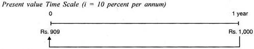
Suppose, for example, you have an opportunity to buy a debenture today and you will get back Rs. 1,000 after one year. What will you be willing to pay for the debenture today if your time preference for money is 10 percent per annum?
We can calculate the present value of Rs. 1,000 to be received after one year at 10% time preference rate as below:
Vn = V0 (1+i)
(Where Vn = Future value n period
and Y0 = Present Value)
or V0 = Vn/(1+i)
1000/1.10
= Rs. 909
The concept of present value can be represented on time scale as shown below:
Present Value or Discount Factor Tables:
We have observed in compounding technique that as n becomes large, the calculation of (1+i)n becomes difficult. To calculate the present values in such cases we can make use of Present Value or Discount Factor Tables.
A potion of the table is reproduced below for ready use:

The discount factor for (i) percent interest and n periods is DFi, n which is equal to 1/(1+i)n
or
DFi, n = 1/(1+i)n
Present value (Vn) = Future Value (Vn) x DFi, n
Illustration 7:
Mr. X is to receive Rs,. 5,000 after 5 years from now. His time preference for money (rate of interest) is 10 percent per annum. Calculate its present value by using discount factor tables.
Solution:
We look to the discount factor tables 10% column and the row for the 5th year. The discount factor is .621.
Percent Value (V0) = Future Value (Vn) x DFi, n
= 5,000 x .621
= Rs. 3,105
Present Value of a Series of Payments:
So far, we have considered only present value of a single payment to be received or paid after a certain period. But in many instances we may have to calculate present value of several sums of money, each occurring at different point of time.
If series of payments is represented by R1, R2, R3 etc. the present value of such a series pf payments will be:
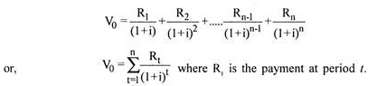
We can also calculate the present value of a series of payments by finding out present values of such individual payments and then adding these present values. It has been explained in the following illustration.
Illustration 8:
Calculate present value of the following cash flows assuming a discount rate of 10%.

Solution:


Present Value of an Annuity:
An annuity is a series of equal payments lasting for some specific period. If the amount of payment is R, the present value of an annuity can be calculated as:
![]()
Using the Annuity Discount Factor Tables, The present value of annuity can be calculated by multiplying the annuity payment with the annuity discount factor.
V0 =(R)(ADFi, n)
Illustration 9:
Mr. X has to receive Rs. 2,000 per year for 5 years. Calculate the present value of the annuity assuming that he can earn interest on his investment at 10% p.a.
Solution:
V0 = (R) (ADFi, n)
In the given question, R = Rs. 2,000
From the Annuity Discount Tables we find that the annuity discount factor at (i), 10 percent and n, 5 years is 3.791
... Present Value (V0) = 2,000 × 3.791
= Rs. 7,582
Present Value of an Annuity Due:
The Present value of an annuity due, i.e. if the cash flows occur at the beginning of each year can be calculated by using the Present Value Tables as below:
V0 = (R)(ADFi, n)(1+i)
Illustration 10:
Mr. A has to receive Rs. 1000 at the beginning of each year for 5 years. Calculate the present value of the annuity due assuming 10% rate of interest.
Solution:
V0 = (R)(ADFi, n)(1+i)
= 1000 [3.791 × 1.10]
= 1000 [4.17]
= Rs. 4170
Present Value of an Infinite Life Annuity:
The present value of an infinite (a) life annuity can be calculated as:
V0 =(R)(ADFi, α) V
or, V0 = R/i
This is because as the length of time of the annuity increases, the discount factors increase, but when the length of time gets very long, this increase in annuity factor slows down. And as it becomes infinitely long the annuity discount factor reaches the upper limit, i.e., 1/i.
Illustration 11:
Calculate the present value of Rs. 1,000 received in perpetuity for an infinite period, taking discount rate of 10%.
Solution:
V0 = R/i
= 1,000/.10 = Rs. 10,000
Present Value of an Annuity Growing at a Constant Rate:
When cash flows grow at a constant rate, we will have to calculate the series of cash flows first and then the present value of the series of payments as demonstrated in the following illustration.
Illustration 12:
Mr. X has rented out a portion of his house for 4 years at an annual rent of Rs. 6,000 with the stipulation that rent will increase by 10 per cent every year. If the required rate of return is 15 per cent, what is the present value of the expected series of rent?
Solution:
