Term Paper on Inventory Management | Firm | Management

Here is a term paper on the ‘Inventory Management in a Firm’ especially written for school and management students.

Term Paper # 1. Objectives of Inventory Management:

The basic responsibility of the financial manager is to make sure the firm’s cash flows are managed efficiently. Efficient management of inventory should ultimately result in the minimization of the owner’s wealth.

In order to minimise cash requirements, inventory should be turned over as quickly as possible, avoiding stock-outs that might result in closing down the production line or lead to a loss of sales. It implies that while the management should try to pursue the financial objective of turning inventory as quickly as possible, it should at the same time ensure sufficient inventories to satisfy production and sales demands. In other words, the financial manager has to reconcile these two conflicting requirements.

Stated differently, the objective of inventory management consists of two counterbalancing parts:

(i) To minimise investment in inventory.

(ii) To meet a demand for the product by efficiently organising the production and sales operations.

These two conflicting objectives of inventory management can also be expressed in terms of cost and benefit associated with inventory. That the firm should minimise investment is inventory implies that maintaining inventory involves costs, such that the smaller the inventory, the lower is the cost of the form.

Inventory ∝ Cost of firm

But, inventories also provide benefits to the extent that these facilitate the smooth functioning of the firm, larger the inventory, the better it is firm this point of view. Obviously, the financial managers should aim at a level of inventory which will reconcile these conflicting elements means, an optimum level of inventory should be determined on the basis of the trade-off between costs and benefits associated with the level of inventory.

A. Cost of Holding Inventory:

One operating objective of inventory management is to minimise cost. Excluding the cost of merchandise.

The costs associated with inventory fall into following two basic categories:

1. Ordering or acquisition or set-up costs.

2. Carrying cost.

These costs are important elements of the optimum level of inventory decisions.

1. Ordering Costs:

This category of costs is associated with the acquisition or ordering of inventory. Firm have to place orders with suppliers to replenish inventory of raw materials. The expenses involved are referred to as ordering costs.

Apart from placing orders outside, the various production departments have to acquire materials from the stores. Any expenditure involved here is also a part of the ordering cost. Ordering cost involves-

Preparing a purchase order or requisition form.

Receiving, inspecting and recording the goods received to ensure both quantity and quality.

The cost of acquiring materials consists of clerical costs and costs of stationary. It is therefore called a set-up cost. These are generally fixed/order placed, irrespective of the amount of the order.

Note:

a. The larger the orders placed, or the more frequent the acquisition of inventory made, the higher are such costs.

b. From a different perspective, the larger the inventory, the fewer are the acquisition and the smaller/lower one the order costs. Acquisition costs one inversely related to the size of inventory. These declines with the level of inventory.

Thus such costs can be minimised by placing fewer orders for a larger amount. But acquisition of a large quantity would increase the cost associated with the maintenance of inventory that is carry cost.

2. Carrying Cost:

The second broad category of cost associated with inventory one the carrying costs. These are involved in maintaining or carrying inventory. The cost of holding inventory or carrying cost.

May be divided into following two categories:

(i) Cost arises due to storing of inventory.

(ii) Opportunity cost of funds.

(i) Cost Arises due to Storing of Inventory:

The main components of this category of carrying cost are:

Storage cost i.e., tax, depreciation, insurance, maintenance of building, utilities and janitorial services.

Insurance of inventory against fire and theft.

Deterioration in inventory because of pilferage, five, technical obsolescence, style obsolescence and price decline.

Servicing costs i.e., labour for handling inventory, clerical and accounting costs.

(ii) Opportunity Cost of Funds:

This consists of expenses in raising funds (interest on capital) to finance the acquisition of inventory. If funds were not looked up in inventory: would have earned a return. This is the opportunity cost of funds on the financial cost component of the cost.

The carrying costs and inventory size are positively related and move in the same direction. If the level of inventory increases, the carrying costs also increase and vice-versa.

Carrying cost ∝ size of inventory. q

Note:

a. The sum of the ordering and carrying costs represents the total costs of inventory.

b. When total cost of inventory is compared with the benefits arising out of the inventory to determine the optimum level of inventory.

B. Benefits of Holding Inventory:

The second element in the optimum inventory decision deals with the benefits associated with holding inventory. The major benefits of holding inventory are the basic function of inventory. In other words, inventories perform certain basic functions which are of crucial importance in the firm’s production and marketing strategies.

The basic function of inventories is to act as a buffer to decouple the various activities of a firm so that all do not have to be pursued at exactly the same rate.

The key activities are as below:

(i) Purchasing.

(ii) Production.

(iii) Selling.

The term uncoupling means that these interrelated activities of a firm can be carried on independently. Without inventories, purchasing and production would be completely controlled by the sales schedules.

If the sales of a firm increase, these two would also increase and vice-versa. Means, purchase and production functions would depend upon the level of sales. It is of course, true that in the long run, the purchasing and production are infact tied to the sales activity of a firm. But, if in the short run, these are rigidly related, the three key activities cannot be performed efficiently.

Inventory/ies permit short term relaxation so that each activity may be pursued efficiently. “Inventories enable firms in the short run to produce at a rate greater than purchase of raw materials and vice-versa or to sell at a rate greater than production and vice-versa.

Since inventory enables uncoupling of the key activities of a firm, each one can be operated at most efficient rate. This has several beneficial effects on the firm’s operations. There are three types of inventories — raw materials, work-in-progress and finished goods, perform certain useful function.

The effect of uncoupling i.e., maintaining inventory are as follows:

1. Benefits in purchasing.

2. Benefits in production.

3. Benefits in work-in-progress.

4. Benefits in sales.

1. Benefits in Purchasing:

If the purchasing of raw materials and other goods is not tied to production/sales means a firm can purchase independently to ensure the most efficient purchase, several advantages would become available.

In the first place, a firm can purchase larger quantities than is warranted by usage in production or sales level. This will enable it to avail of discounts that are available on bulk purchases.

Moreover, it will lower the ordering cost as fewer acquisition would be made. There will, thus be a significant saving in the costs.

Secondly, firms can purchase goods before anticipated or announced price increases. This will lead to decline the cost of production.

Inventory, thus, serves as a hedge against price increases as well as shortages of raw materials. This is a highly desirable inventory strategy.

2. Benefits in Production:

Finished goods inventory severs to uncouple production and sale. This enables production at a rate different from that of sales, i.e., production can be carried on at a rate higher or lower than the sales rate. This would be of special advantage to firms with seasonal sales pattern. In this case, the sales rate will be higher than the production rate during a part of the year i.e., peak season and lower during the off season.

The choice with the firm is either to produce at a level to meet the actual demand that is higher production during peak season and lower or nil production during off season or produce continuously throughout the year and build up inventory which will be sold during the period of season demand.

The farmer involves discontinuity in the production schedule while the latter ensures level production. The level production is more economical as it allows the firm to reduce the cost of discontinuities in the production process.

This is possible because excess production is kept as inventory to meet the future demands. Thus inventory helps a firm to coordinate its production scheduling so as to avoid disruption and the accompanying expenses.

Note:

Inventory permits least cost production scheduling, production can be carried or more efficiently.

3. Benefits in Work-in-Progress:

Inventory of work-in-progress perform following in functions.

It is necessary because production processes are not instantaneous. The amount of such inventory depends upon technology and the efficiently of production. The larger the step involved in the production process, the larger the work-in-progress inventory and vice-versa.

Number of steps in production process ∝ WIP inventory

By shortening the production time, efficiency of the production process can be improved and the size of this type of inventory reduced.

In the multi-stage production process it uncouples the various stages of production so that all of these do not have to perform at the same rate. The stages involving higher set-up costs may be most efficiently performed in batches with a W.I.P inventory accumulated during a production run.

4. Benefits in Sales:

The maintenance of inventory also helps a firm to enhance its sales efforts.

If there are no inventories of finished goods, the level of sales will depend upon the level of current production. A firm will not be able to meet demand instantaneously. There will be a log depending upon the production process.

If the firm has inventory, actual sales will not have to depend as lengthy manufacturing processes. Thus, inventory serves to bridge the gap between current production and actual sales.

A related aspect is that inventory serves as a competitive marketing tool of meet customer demands. A basic requirement in a firm’s competitive position is its ability vis-a-vis its competitions to supply goods rapidly. If it is not able to do so, the customers are likely to switch to supplier who can supply goods at short notice.

Note:

a. Inventory thus ensures a continued patronage of customers.

b. In case firm having a seasonal pattern of sales, there should be a substantial finished goods inventory prior to the peak sales season, failure to do so may mean a loss of sales during the peak season.

Term Paper # 2. Inventory Management Techniques:

Financial managers should aim at an optimum level of inventory on the basis of trade-off between costs and benefit to maximise the owner’s wealth. Many sophisticated mathematical techniques are available to handle inventory management problems. Following are a few simple production-oriented methods/techniques of inventory control to indicate a broad framework for managing inventories efficiently in conformity with the good of wealth maximization.

The major problems areas that comprise the heart of inventory control are:

1. Classification problem to determine the type of control required.

2. The order quantity problem.

3. The order point problem.

4. Safety stocks.

1. Classification Problem—ABC System:

The first step in the inventory control process is classification of different types of inventories to determine the type and degree of control required for each.

The ABC system is a widely used classification technique to identify various items of inventory for purposes of inventory control. This technique is based on the assumption that a firm should not exercise the same degree of control on all items of inventory.

It should rather keep a more rigorous control on items that are:

(i) The most costly.

(ii) Slowest turning.

While items that are less expensive should be given less control efforts.

On the basis of cost involved, the various inventory items are, according to this system, categorised into following three classes:

i. Class A.

ii. Class B.

iii. Class C.

The items included in class A’ involve the largest investment. Therefore, inventory control should be the most rigorous and intensive and the most sophisticated inventory control techniques should be applied to these items.

The class ‘C’ consists of items of inventory which involve relatively small investment although the number of items is fairly large. These items deserve minimum attention.

The class ‘B’ stands midway. It deserves less attention than ‘A’ but more than ‘C’. It can be controlled by employing less sophisticated techniques.

The take of inventory management is to properly classify all the inventory items into one of these three categories/classes.

The typical break down of inventory items is as below:

Notes:

a. Class ‘A’ is the least important in term of the number of items; it is by far the most important in terms of the investment involved. With only 15% of the number, it accounts for as much

as 70% of the total value of inventory. The firm should direct most of its inventory control efforts to the items included in this group.

b. The items comprising ‘B’ class account for 20% of the investments in inventory. Class ‘B’ deserves less attention than ‘A’ but more than ‘C’.

c. Class ‘C’ involves only 10% of the total value although number wise its share is as high as 55%.

Example 1:

A firm has 7 different items in its inventory. The average number of each of these items held, along with their unit costs is as below. The firm wishes to introduce ABC inventory system. Suggest a breakdown of the items in ABC system.

Solution:

ABC analysis:

Item 1 and 2 combine together are of 15% whereas cost % is 70, hence are placed in class ‘A’. Items 3 and 4 combine together are of 30% whereas cost % is 20, hence are placed in class ‘B’. Items 5, 6 and 7 combine together are of 55% whereas cost % is 10, hence are placed in class ‘C’.

Note:

Though ABC classification is quite simple but must use with caution. At times an item may be very expensive but very critical in the process of production.

Advantages of ABC analysis:

The advantages of ABC analysis are as follows:

i. It becomes possible to concentrate all efforts in areas which need genuine efforts.

ii. This method produces rewarding results, at the same time it involves minimum control.

iii. In respect of class ‘A’ items care attention is paid at every step i.e., estimates of requirements, purchasing, safety stock, receipts, inspection, issues etc. A tight and lose control is exercised. A close watch on high consumption items and their progress of replenishment use etc., is maintained. But ‘C’ class items, which are numerous and at the same time inexpensive one comparatively left loose controlled.

4iv. Those items which fall under class ‘C’ may be dispersed with in the record-keeping system as well, physical division of these items into two unequal sections may help in saving time, money and labour without endangering the production schedule.

v. It is the most effective and economical method as it is based on selective approach.

vi. It helps in placing the order. Deciding the quantity of purchase, safety stock etc. Thus saving the enterprise/firm from unnecessary stock cuts or surpluses and their resultant consequences.

ABC Analysis Pattern:

The control on inventories under selective approach may follow the following pattern:

Broad Policy Differences between ABC Items:

ABC analysis is carried with an object of evolving policy guidelines for selective materials control under the method. For an effective and purposeful analysis policy guidelines are based on differences between the three – ABC types of items.

A broad policy guideline may be established and followed. The establishment of such guidelines may help in achieving the objects which the ABC method of inventory classification sets for itself. The objects of the method may be enumerated as the broad policy differences or guidelines which are easy to evolve once materials are classified as ABC items.

Following table shows the broad policy difference between the three classes of items:

Limitation of ABC Analysis:

This analysis is not foolproof. It suffers from certain limitations which later methods have tried to remove.

The limitations are as below:

i. It can achieve its objectives only when there is a popular standardization of materials being carried in the store house. A good system of codification two is required for effectively carrying out the analysis.

ii. The base of ABC analysis is “grading of items” carried in the store house. The grading of items is done according to the importance of performance of the item under gradation. The gradation of item is obviously done on the basis of vital (V), Essential (E) and desirable (D). Vitality, essentiality and desirability of the items speak for themselves and any analysis has to be based on these. Any item may be having zero or minimum monetary value but may be vital for the functioning of organizations smoothly and efficiently.

iii. The inventory position may be analysed according to the value of the item. Thus a periodic review and updating is mandatory in ABC analysis.

iv. ABC analysis which primarily based on monetary value of the item ignoring other important factors.

v. Despite the above limitation, still the ABC analysis is an effective tool and serves very useful purposes.

VED Analysis:

It is quite similar to ABC analysis but largely applicable to spare parts. Spare parts are classified as Vital, Essential and Desirable according to their requirement.

Spares classified as ‘V’ (vital) are stocked adequately to ensure smooth plant operations. These spares are those which may cause havoc and may amount to stoppage work in the organization if are not available at the time of requirement.

However, the organization may take a reasonable risk in case of those spares which are classified as ‘E’ (Essential). These items can be sufficiently stocked to ensure a regular flow but care should be taken that if sufficient stock of ‘E’ items is not available then it may affect the efficiency of the organisation. Therefore, it is necessary to have adequate arrangement for their replenishment at a short notice.

The suppliers of ‘E’ items should be reliable and should be such who may be ready to supply the items as and when needed. ‘D’ (Desirable) spares are those which can be easily bought from the market as and when these are needed. The lead time of such items is always low and their procurement at any time or at any stage is not going to face any problem.

VED classification is helpful to those industries which largely depend on their plant and machinery.

Note:

a. Use of VED analysis is most advantageous in the capital intensive industries.

b. Transport industry should invariably option for VED an analysis. P. Gopala Krishanan and MS Sandilya have suggested a combination of ABC and VED analysis in order to control the stacking of spare parts.

According to them control action may be classified as AV, BE and CD. They are of the opinion that in such cases it will be advantageous to have a centralised system of storage so far as the spare parts are concerned, particularly an undertaking which is organised as multi-unit organisation.

Pattern of ABC-VED Analysis:

FSN Analysis:

It is based on movement of item from and in the store. The items are classified as ‘F’ (fast moving, ‘S’ (slow moving) and ‘N’ (non-moving). The classification is based upon the movement/ consumption pattern of the items under analysis. This analysis is useful in case of obsolete items. Previous year’s issue is the guiding factor for FSN analysis. Previous 2-3 years consumptions are taken into consideration for decision. Whether the items stocked in store are fast moving, slow moving or non-moving.

Certainly, such analysis and method of analysis is useful in locating and identifying the obsolete items.

This analysis helps in avoiding investments is non-moving or slow moving items. FSN analysis is also useful in presenting obsolescence and facilities timely control.

2. Order Quantity Problem:

Economic Order Quantity (EOQ) Model:

After various inventory items are classified on the basis of suitable analysis, the management becomes aware of the type of control that would be appropriate for each of class of inventory items.

A key inventory problem while purchasing raw materials or finished good, how much inventory should be purchased/bought in one lot under one order on each replenishment? Should the quantity to be purchased be large or small? or should the requirement of materials during a given period of time be acquired in one lest or should it be acquired in installments or in several small lots? Such inventory problems are called order quantity problems.

The determination of the appropriate quantity to be purchased in each lot to replenish stock as a solution to the order quantity problem necessitates resolution of conflicting goals.

Note:

a. Buying a large quantity implies a higher average inventory level which will assure.

(i) Smooth production/sales operation, and

(ii) Lever ordering or set up casts. But will involve higher carrying cost.

b. Small orders would reduce the carrying cast of inventory by reducing the average inventory level but the ordering casts would increase as there is a livelihood of interruption in operations due to stock run arts.

A firm should place neither too larger nor too small orders. On the basis of tradeoff between benefits derived firm the availability of inventory and the cost of carrying that level of inventory, the appropriate or optimum level of the order to be placed should be determined.

The optimum level of inventory is popularly referred to as the Economic Order Quantity [EOQ], It is also known as economic lot size.

The Economic Order Quantity [EOQ] may be defined as the level of inventory order that minimises the total cost associated with inventory management.

The costs associated with inventories are:

(i) Ordering costs.

(ii) Carrying cost.

EOQ refers that level of inventory at which the total cost of inventory comprising acquisition/ ordering/set-up costs and carrying cost is minimal.

Assumption for EOQ:

The EOQ model, as the technique to determine the economic order quantity is based upon following three restrictive assumptions:

1. The firm known with certainty the annual usage (consumption) of a particular item of inventory.

2. The rate at which the firm uses inventory is steady over time.

3. The orders placed to replenish inventory stocks are received at exactly that point in time when possible inventory levels being considered.

Approaches:

The EOQ model can be understood by:

(i) Long analytical approach or trial and error approach.

(ii) The shortcut or simple mathematical approach.

(i) Long analytical/trial and error approach:

Given the total requirements of inventory during a given period of time depending upon the inventory planning horizon, a firm has different alternatives to purchase its inventories like:

It can buy its entire requirements in one single lot at the beginning of the inventory planning period.

The inventories may be procured in small lots periodically.

If the purchases are made in one lot, the average inventory holdings would be relatively large whereas it would be relatively small when the acquisition of inventory is in small lots. The smaller the lot the lever is the average inventory and vice-versa.

Lot size ∝ average inventory

High average inventory would involve high carrying costs:

On the other hand, low inventory holdings are associated with high ordering cost:

The trial and error or long analytical approach for the determination of EOQ uses different permutations and combinations of lots of inventory purchases so as to find at the least acquisition costs for different sizes of orders to purchase inventories are computed and the order size with the lowest total cost i.e., ordering plus carrying of inventory is the economic order quantity.

The mechanics of the computation of EOQ with the analytical approach is as follows:

Example 2:

A firm’s inventory planning period is one year. Its inventory requirement for this period is 1600 units. If the acquisition cost is Rs.50 per order. The carrying costs are expected to be Re. 1 per unit/year for an item.

The firm can procure inventories in various lots as below:

(i) 1600 units,

(ii) 800 units,

(iii) 400 units,

(iv) 200 units, and

(v) 100 units.

Which of these order quantities is the EOQ.

Solution:

Inventory Costs for Different Order Quantities:

Working notes:

(i) No. of orders = Total inventory requirements/order size.

(ii) Average inventory = Order size/2.

From the above total cost it reveals that-

The carrying and ordering costs when taken together are the lowest for the ordering size of 400 units hence it is the EOQ.

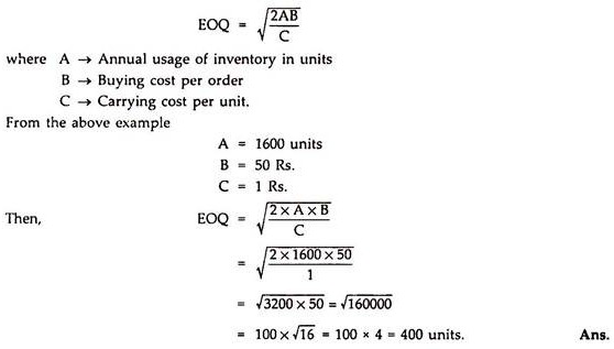
(ii) Mathematical Approach (Shortcut Method):

The economic order quantity can, using a shortcut method, be calculated by the following formula.:

Limitations:

It suffers from short comings due to the restrictive nature of the assumptions.

i. The assumption of a constant consumption/usage and the instantaneous replenishment of inventory is of doubtful validity. Deliveries from suppliers may be slower than expected for reasons beyond control. It is also possible that there may be an unusual and unexpected demand for stocks. To meet such contingencies, firms have to keep additional inventories which are known as safety stocks.

ii. Assumption of a known annual demand for inventories is open to question. There is likelihood of a discrepancy between the actual and the expected demand, leading to a wrong estimate of EOQ.

iii. In addition, there are same computational problems involved. A more difficult situation may over when the number of orders to be placed may turn out to be a fraction.

3. Order Point Problem:

The EOQ technique determines the size of an order to acquire inventory so as to minimise the carrying as well as the ordering costs. In other words EOQ provides an answer to the question. How much inventory should be ordered in one lot? Another important question pertaining to efficient inventory management is when should the order to procure inventory be placed? It is known as reordering point.

Reordering point is stated in terms of the level of inventory at which an order should be placed for replenishing the current stock of inventory. In other words, reorder point may be defined as the level of inventory when fresh order should be placed with the suppliers for procuring additional inventory equal to the economic order quantity.

A simple formula to calculate the reorder point is based upon following assumptions:

(i) Constant daily usage of inventory.

(ii) Fixed lead time.

In other words, the formula assumes conditions of certainty.

The reorder point = lead time in days × average daily usage of inventory.

or

ROP = LT × ADU.

OP_R or L × U.

Where ROP or OP_R = Recording point

LT or L = Lead time in days.

ADU or U = Average daily usage of inventory lead time refers to the time normally taken in receiving the delivery after placing orders with the suppliers. It covers the time span from the point when a decision to place the order for the procurement of inventory is made to the actual receipt of the inventory by the firm.

In other words the lead time consists of number of days required by the supplier to receive and process the order as well as the number of days during which the goods will be in transit from the supplier. The lead time may also be called as the procurement time of inventory.

The average usage means the quantity of inventory consumed daily. Therefore, reorder point can be defined as the inventory level which should be equal to the consumption during the lead time.

4. Safety Stock:

The economic order quantity and the reorder point are on the assumption of certainty conditions i.e.,

(i) Constant/fixed usage/ requirement of inventory.

(ii) Instantaneous replenishment of inventory.

These assumptions are subjected to questionable validity in central conditions/situations. For instance, the demand for inventory is likely to fluctuate from time to time. In particular, at certain points of time the demand may exceed the anticipated level. In other words, a discrepancy between the assumed or estimated or anticipated or expected and actual usage rate of inventory is likely to occur in practice. Similarly, the receipt of inventory from the suppliers may be delayed beyond the expected/pre calculated lead time.

The delay may arise from strikes, floods, transportation and other unforeseen bottlenecks. Thus, a firm would come across situations in which the actual usage of inventory is higher than the anticipated level and/or the delivery of the inventory from the supplier is delayed.

The effect of increased and/or slower delivery would lead to shortage of inventory. That is, the firm would face a stock-out situation. This would disrupt the production schedule and reduce the customers. The firm would, therefore, be well advised to keep a sufficient safety margin by having an additional inventory to guard against stock-out situation. Such stocks are called safety stocks.

This safety stocks act as a buffer or cushion against stock-out situation/possible shortage of inventory caused either by increased usage or delayed delivery of inventory.

The safety stock may be defined as the minimum additional inventory to serve as a safety margin or buffer or cushion to meet an unanticipated increase in usage resulting from an unusually high demand and or an uncontrollable late receipt of incoming inventory.

The safety stock involves two types of costs:

(i) Stock-out.

(ii) Carrying cost.

The job of working capital manager is to determine the appropriate level of safety stock on the basis of trade-off between these two above discussed conflicting costs.

The stock-out costs refers to the cost associated with the shortage (stock-out) of inventory, the firm would be deprived of certain benefits. The denial of those benefits which would otherwise be available to the firm are the stock-out costs.

The first and most important of these costs, is the loss of profit. Which the firm could have earned from increased sales if there was no shortage of inventory.

Another category of stock-out-costs is the damage to the relationship with the customers. Owing to shortage of inventory, the firm would not be able to meet the customer’s requirements and the latter may turn to the firm’s competitions. It should of course be clearly understood that this type of cost cannot be easily and precisely quantified.

Last, the shortage of inventory may disrupt the production schedule of the firm. The production process would grind to a halt involving idle time.

The carrying costs are the costs associated with the maintenance of inventory. Since the firm is required to maintain additional inventory, in evens of the normal usage, additional carrying costs are involved.

The stock-out and the carrying costs are counter balancing. The longer the safety stock the larger would be the carrying cost and vice-versa.

Safety stock ∝ carrying cost.

Larger is the safety stock, the smaller would be the stock-out-costs.

Safety stock 1/∝ stock-out-costs.

In other words, if the firm minimises the carrying cost the stock-out-costs are likely to rise, on the other hand, an attempt to minimise the stock-out-costs implies to increase carrying costs.

The object of the working capital manager should be to have the lowest total cost i.e., carrying cost + stock-out-costs.

The safety stock with the minimum carrying and stock-out costs is the economic or appropriate level which a working capital manager should aim at.

The appropriate level of safety stock is determined by the trade-off between the stock-out and the carrying costs.