This article throws light upon the top four economic principles applied to farm management. The economic principles are: 1. The Law of Diminishing Marginal Returns 2. The Law of Equi-Marginal Returns 3. Law of Opportunity Cost 4. Law of Comparative Advantage.
Economic Principle # 1. The Law of Diminishing Marginal Returns:
Since agriculture is a productive activity we should be well versed with the process of production. Production is defined as transformation of two or more inputs (resources) into one or more products. The farm resources are land, labour, capital, organization (management), enterprise.
The per unit return from the factors of production is called ‘productivity’. Total output is called ‘production’. The relationship between input and production is called ‘Input-output’ relationship. There are different ways in which resources can combine and substitute for one another in the production process.
This is input-input i.e., Factor-Factor relationship. The relationship between different products which can be produced is known as ‘Output-output’ i.e., Product- Product relationship. Thus, there are three clear-cut relationship, viz., Factor-Product; Factor-Factor and Product-Product.
ADVERTISEMENTS:
In the sciences of production economics and farm management, under the Laws of Returns there are total products, average products and marginal products. These concepts are very important and should be well understood.
The total product is the amount of product which is the result of different amounts of variable inputs used.
Average product is the result of total product at a particular level of input used divided by the level of input used.
Marginal product is the quantity which is produced by the last unit of the variable input used.
ADVERTISEMENTS:
Expressed symbolically:
Y = total product;
X = input;
T/Y = Average product;
ADVERTISEMENTS:
∆Y/∆X = Marginal product;
∆ = the change in Y and X.
There is a definite relationship between total, average and marginal products in the production:
(a) When TP is maximum, MP is zero.
ADVERTISEMENTS:
(b) When TP is zero, AP is zero.
(c) If AP is maximum, the ratio of output to input is maximum = MP = AP.
(d) When MP is at its maximum, TP is at the point of inflection.
(e) When AP is increasing, MP > AP.
ADVERTISEMENTS:
(f) When AP is decreasing, MP < AP.
There is the algebraic proof of the relationship between TP, AP and MP:
TP = Y; Input X; AP = Y/X; MP = dY/dX
(a) For rising AP:dY/dX or, MP > AP
ADVERTISEMENTS:
(b) For the maximum AP: dY/dX= Y/X or, MP = AP.
(c) For decreasing AP: dY/dX = Y/X or, MP <AP
(d) TP is maximum when, dTP/dX1 = 0 (Zero)
ADVERTISEMENTS:
That is, MP = 0, when TP is maximum
or, dY/dX = 0 or, Mp = 0 =0 or, MP = 0
MP is at the maximum, when TP is at the point of inflection.
The significance of MP (Marginal product):
(a) When MP is increasing, TP increases at an increasing rate.
ADVERTISEMENTS:
(b) When MP is decreasing, but is more than zero. TP increases at a decreasing rate.
(c) When MP is zero, TP is at its maximum.
(d) When MP is greater than AP, AP is increasing.
(e) When MP is less than AP, AP is decreasing.
(f) When MP is equal to AP, AP is at its maximum.’
Principles of Diminishing Returns:
ADVERTISEMENTS:
The Principles of Diminishing Returns or the Law of Diminishing Marginal Returns is highly applicable in decision-making under the farm management. This law is defined as “an increase in capital and labour employed in the cultivation of land causes, in general, a less than proportionate increase in the amount of produce raised unless it happens to coincide with an improvement in the art of agriculture.”
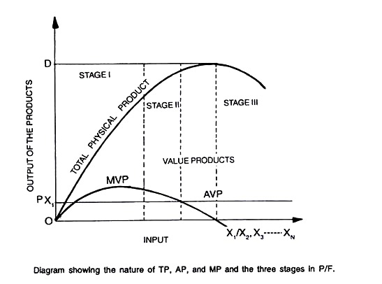
This is the definition given by Alfred Marshall. This law establishes an input- output relationship, which applies very fast in agriculture. This is a case of physical input-output relationship. This relationship is also called FACTOR-PRODUCT relationship and technically known as “PRODUCTION FUNCTION” which means that the output is a function of input. Algebraically expressed is: Y = f(X1 X2………………. Xn). A close examination of the given diagram shows the relationship as already mentioned in the foregoing pages.
But further explanation is:
TP is a total output as a result of the application of a single (in case of one variable study) or several inputs (in case of multiple variables). The shape of the production function curve is governed by the elasticity of production as a result of inputs.
Here AP and TP are interrelated. The shape of MP curve depends on the law of diminishing returns, i.e., in relation to the fixed inputs what returns it can give. This is a very important concept in production economics. Let us examine the three stages in the production function (Law of diminishing marginal returns).
These three stages are demarcated as:
ADVERTISEMENTS:
(a) Stage I:
It extends from the point of origin (The juncture of OX and OY axis’s) where AP is maximized and MP = AP. At this point MP curve crosses AP curve demarcating the stage I from II.
Stage II:
It starts from the point where AP is at the maximum and ends where MP is zero. The boundary of this stage is at the point of maximum TP and zero MP. This is called RATIONAL STAGE. Why ? Because, MP though decreasing is not negative.
If we put the price of output and input price, the profit will be the maximum where MC = MP. But with a change in product and input unit prices there will be a shift in the equivalence of MC and MP.
Stage III:
ADVERTISEMENTS:
This point starts from where MP is zero, after this MP is less than zero and TP decrease. It is a stage of negative MP. Stage I and III are called irrational stages, because in stage I, AP and MP are increasing and MP is always greater than AP therefore if more inputs are used it will add output in greater proportion.
In stage m since MP is less than zero the additional input will give less and less output. The total profit starts diminishing.
The algebraic expression of these stages are:
Elasticity of Production, (Ep):
Expressed another way, by definition Y/X = AP, and ∆Y/∆X = MP therefore, Ep = MP/AP.
ADVERTISEMENTS:
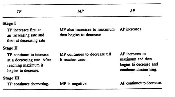
Properties of the TP, AP, & MP, under each of the three stages.
Economic Principle # 2. The Law of Equi-Marginal Returns:
As we know that the farm managers work under two situations as regards the capital viz., either under unlimited resources or under limited resources. The law of equi-marginal returns works or is applicable under limited resources. Under the capital constraints the farmer, for instances, Rs. 5,000 to use for two enterprises Y1 and Y2. He has the option of using a doze of Rs. 1,000 for both the enterprises.
This will illustrate the law of diminishing returns as it applies in the input-output relationship. The law of equi-marginal return states that “the profits are maximized by using the resource in such a way that the marginal returns from the resources are equal in all cases.”
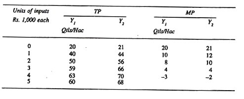
In the following illustration we will take only TP and MP into consideration:
In the above illustration we see that with the option of using only five doses of inputs package we see that in Y1 after the application of two doses and in Y2 with the application of three doses the marginal productivity are 10 each respectively.
This satisfies the law that the outputs are equi-marginal in returns. Let us examine the case with further manipulation that is, by using different doses but only five for each product.
If we increase the doses in Y1, the MP will be 9 and we will have to use only two doses in Y2 for which MP will be 12 or we can apply four doses to Y1 and left to apply only one in case of Y2. Let us see what is the total gain in the three cases.
With 2 and 3 doses in Y1, and Y2 we get 73, in second case we get 72, and in the third case we get only 64. Therefore, by adhering to this law the farmer can get highest return than by ignoring this law. This illustration gives return in physical terms.
If we are interested in economic returns the physical returns must be converted into value terms then we see that the last rupee in each is equal in order to maximize profit, that is,
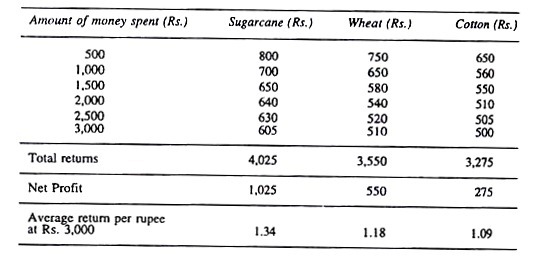
Another illustration will give a clear picture of what we get, when we apply this law in terms of total returns, net profit and average return per rupee from the total allocated fund.
The farmer has Rs. 3,000 at his disposal using a dose of 500 rupees. He has an option of using them in three enterprises viz., sugarcane, wheat, and cotton. Let us see how judiciously the farmer uses his limited fund.
Addition to Income from the Marginal Amount of Rs. 5000 each.
Now, the option is to choose between average return or equi-marginal return. From the figure it is the equi-marginal return which is the best. With the equi-marginal return Rs. 3,000 should be used in total for each enterprise as Rs. 1,500 for sugarcane, Rs. 1,000 for wheat, and Rs. 500 for cotton, i.e.,
PY1, (Y1,/X) = PY2 (Y2/X)……………….. = PYn (Yn/Xn Px)
That, the marginal productivity of rupee in each case be equal.
Practical Utility of the Law of Equi-marginal Returns:
1. Planning of the farmer’s budget.
2. Determining enterprise relationship as complementary, or competitive.
3. Guidance for diversification or specialization in farming.
Economic Principle # 3. Law of Opportunity Cost:
The opportunity cost is a concept wherein earning from the next best alternative is not availed. An example will make it clear, in the Rabi season wheat and potato could be raised on one hectare of land available with the farmer.
Potato cultivation can yield a profit of Rs. 10,000 and wheat Rs. 8,000. Other things remaining the same, the farmer will put the land under potato foregoing wheat which is the second best alternative.
Opportunity cost are calculated by two methods:
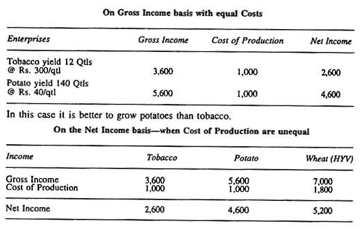
(a) On gross income basis-when cost of production are equal.
(b) On net income basis-when cost of production are not equal.
Illustration:
In this case, the net income generated by the three crops, tobacco, potato, and wheat are Rs. 2,600, Rs. 4,600, and Rs. 5,200 respectively. It is, therefore, wise to cultivate wheat as it gives the highest net income.
Economic Principle # 4. Law of Comparative Advantage:
In the wake of globalization and open economy and encouragement to agricultural sector to enter into the arena of international trade. We are making efforts to export the agricultural commodities to the nation outside India.
For this, the understanding of the basis of international trade, of which the law of comparative advantage, is very important. We have already explained the concept and theory in connection with the law of comparative advantage.
The principles of comparative advantage is based on the differences in production costs of similar commodities in different countries or within the country in different regions, The cost differences are the result of differences in the efficiency of labour and specialization in production.
Specialization depends on the type of farming which is related to climate, natural resources, geographical situation and the efficiency of labour. The trade will take place only when one region or country produces the commodity at a lower cost for which the other region or country has disadvantage.
To cite an example, in paddy cultivation in one region the climate is highly favourable and the labour is cheaper to another region in terms of favourable climate and labour being costly.
Naturally, the cost per unit of output in region A will be lower than that of region B. Thus, the region B will import and region A will export. The farmers of region will specialize in paddy cultivation.
If the region B has comparative advantage in the production of wheat then it will export wheat to region A and region A will import wheat. As it has disadvantage in production of wheat. The country A will specialize in the production of paddy and region B in the production of wheat.
Principles of Combining Enterprises:
In the process of production under all the three situations, viz., factor-product, factor-factor, and product-product relationship we see the production function curve : in the case of factor-product relationship, iso-cost curve in case of factor-factor relationship, and iso-product curve in. case of product-product relationship. It, therefore, becomes necessary to study the elasticity concept.
The elasticity is defined as “the percentage change in the quantity of output per unit of input (F/P relationship), quantity change in input replaced by one unit of input substitute (F/F relationship) and quantity of output changed by the substitution of one unit of the other product,” (P/P relationship).
There are two extremes of elasticity:
Elastic and the other inelastic. While calculating the elasticity we take into consideration two types of elasticity:
(a) Point elasticity;
(b) Arc elasticity.
In the case of F/P relationship we have already discussed the elasticity of
In case F/F relationship, with two inputs X1, and X2, a change in the quantity of X1, from X11 , to X12 will affect the change in X2 from X1 to X22. In order to calculate the elasticity dX1/X will be divided by dX2/X2 that is, one unit change in input X, will bring about a change in X2. The ratio of these two input will express the elasticity of substitution.
The elasticity of substitution will depend on the slope of the curve.
In order to get to the optimum level of the combination of the two inputs we will have to calculate the MRS (Marginal rate of substitution of the two input and compare the same with the price ratio of the two inputs PX1/PX2.
Thus, in order to come or attain the level of optimum combination of the two inputs the MRS = Price ratio.
dX1/X1, – dX2/X2 = PX1/PX2
In case of P/P relationship we shall study the marginal rate of substitution of the two products and compare it will the price ratio of the products:
dY1/Y1: dY2/Y2 will give MRS of Y1, and Y2 and Price ratio of Y1, and Y2 or py1/py2.
When MRS of products will be equal to the price ratio of the two products then optimum combination of the two products will be achieved. This optimum levels will give least cost combination and maximum profit of input and output.
In order to achieve the best combination of enterprises whatever enterprises we are raising on the farm their MRS and Price ratios should be equal. This will give the best combination of enterprises and the farmer will get the maximum profit from the farm business.


